统计计算——Bootstrap总结整理

Bootstrapping

Boostrap 有放回的重抽样。

符号定义： 重复抽样的bootstrap \(F^*\) 观测到的样本\(\hat F\),是一个经验分布
真实分布\(F\)

Eg.
有一个要做估计的参数\(\alpha\)
用原始样本做估计的估计值\(\hat \alpha\)
用重抽样样本做估计的估计值\(\hat \alpha^*\)
重复抽样的bootstrap \(\bar \alpha^* = E(\hat \alpha^*)\)

Bootstrapping generates an empirical distribution of a test statistic or
set of test statistics. 有放回的重抽样。 Advantages:It allows you to
generate confidence intervals and test statistical hypotheses without
having to assume a specific underlying theoretical distribution.

1. Randomly select 10 observations from the sample, with replacement
   after each selection. Some observations may be selected more than
   once, and some may not be selected at all.
2. Calculate and record the sample mean.
3. Repeat steps 1 and 2 a thousand times.
4. Order the 1,000 sample means from smallest to largest.
5. Find the sample means representing the 2.5th and 97.5th percentiles.
   In this case, it's the 25th number from the bottom and top. These
   are your 95 percent confidence limits

What if you wanted confidence intervals for the sample median, or
the difference between two sample medians?

When to use ? - the underlying distributions are unknown - outliers
problems - sample sizes are small - parametric approach don't exist.

Bootstrapping with R

1. Write a function that returns the statistic or statistics of
   interest. If there is a single statistic (for example, a median),
   the function should return a number. If there is a set of statistics
   (for example, a set of regression coefficients), the function should
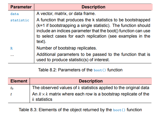
   return a vector.
2. Process this function through the boot() function in order to
   generate R bootstrap replications of the statistic(s).
3. Use the boot.ci() function to obtain confidence intervals for the
   statistic(s) generated in step 2.

library(boot)
#bootobject <- boot(data=, statistic =, R=, ...)
#boot.ci(bootobject , conf= ..., type = ...)

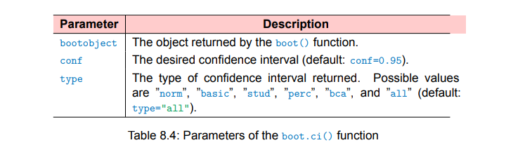
The bca provides an interval that makes simple adjustments for bias.
I find bca preferable in most circumstances.

#indices <- c[3,1,4,1]
# data[c(3,1,4,1)]
my_mean <- function(x,indices){#这个函数的返回值：要估计的统计量。
  mean(x[indices])
}
x <- iris$Petal.Length
library(boot)
boot(x, statistic = my_mean, R = 1000)

• std. error: std of
  \(\hat{\mu_1^*}, \hat{\mu_2^*}...\hat\mu_{R=1000}^*\)
• bias: 重抽样样本均值估计值和原始抽样值的差异。\(E(\hat\mu^*) - \hat \mu = \bar \mu^* - \hat \mu\)
• original:\(\hat \mu\),原始抽样估计值

Bootstrapping for an arbitrary parameter

Eg. Financial assets

Bootstrap for an arbitrary parameter
Example (Financial assets)

• Suppose that we wish to invest a fixed sum of money in two financial assets that yield returns of \(X\) and \(Y\), respectively, where \(X\) and \(Y\) are random quantities.
• Invest a fraction \(\alpha\) of our money in \(X\), and invest the remaining \(1-\alpha\) in \(Y\).
• Minimize

\[\operatorname{Var}(\alpha X+(1-\alpha) Y), \]

and we have

\[\alpha=\frac{\sigma_Y^2-\sigma_{X Y}}{\sigma_X^2+\sigma_Y^2-2 \sigma_{X Y}}, \]

where \(\sigma_X^2=\operatorname{Var}(X), \sigma_Y^2=\operatorname{Var}(Y)\) and \(\sigma_{X Y}=\operatorname{Cov}(X, Y)\)

Question:

How to estimate \(\alpha\), and what is the standard error this estimator?

Solution:

Solution

• In reality, \(\sigma_X^2, \sigma_Y^2\) and \(\sigma_{X Y}\) are unknown.
• Compute estimates for these quantities: \(\hat{\sigma}_X^2, \hat{\sigma}_Y^2\) and \(\hat{\sigma}_{X Y}\).
• Estimate \(\alpha\) by

\[\hat{\alpha}=\frac{\hat{\sigma}_Y^2-\hat{\sigma}_{X Y}}{\hat{\sigma}_X^2+\hat{\sigma}_Y^2-2 \hat{\sigma}_{X Y}} . \]

Estimate the accuracy of \(\hat{\alpha}\).

If we know the distribution of \((X, Y)\)

• Resample \((X, Y) 1000\) times, and calculate \(\hat{\alpha}\) using the same precedure.
• Then, the estimtor for \(E(\hat{\alpha})\) is

\[\bar{\alpha}=\frac{1}{1000} \sum_{r=1}^{1000} \hat{\alpha}_r \]

• The estimator for the standard deviation of \(\hat{\alpha}\) is

\[s=\sqrt{\frac{1}{1000-1} \sum_{r=1}^{1000}\left(\hat{\alpha}_r-\bar{\alpha}\right)^2} \]

If we do not know the distribution of \((X, Y)\)

• Usually, we don't know the distribution of \((X, Y)\). Resample \(\left(X^*, Y^*\right) 1000\) times from the original sample, and calculate \(\hat{\alpha}^*\) using the same precedure.
• Then, the estimtor for \(E(\hat{\alpha})\) is

\[\bar{\alpha}^*=\frac{1}{1000} \sum_{r=1}^{1000} \hat{\alpha}_r^* \]

• The estimator for the standard deviation of \(\hat{\alpha}\) is

\[s^*=\sqrt{\frac{1}{1000-1} \sum_{r=1}^{1000}\left(\hat{\alpha}_r^*-\bar{\alpha}^*\right)^2} \]

总体的\(\sigma_{X}, \sigma_{Y}, \sigma_{XY}\)都可以用样本的来估计。

\[\hat \alpha = \frac{\hat{\sigma_{y}^2} - \hat{ \sigma_{XY}}}{\hat{\sigma_{X}^2} + \hat{\sigma_{Y}^2} - 2 \hat{\sigma_{XY}}} \]

问题在于，这个估计是有偏的，因为除了一些东西在下面，就不是线性的了。

注意在抽样时X,Y两者是一一对应的。

偏差的计算：\(E(\hat \alpha) - \alpha\) -> \(\bar{\alpha*} - \hat{\alpha}\)

两页ppt上的公式s里面都少了个平方。这里补上了。

alpha.fn = function(data, index) {
  X = data$X[index]
  Y = data$Y[index]
  alpha.hat = (var(Y) - cov(X, Y)) / (var(X) + var(Y) - 2 * cov(X, Y))
  return(alpha.hat)
}
library(ISLR2)
alpha.fn(Portfolio, 1:100) # alpha.hat

set.seed(1)
alpha.fn(Portfolio, sample(100, 100, replace = TRUE)) # alpha.hat* # run R=1000 times, we will have E(alpha.hat)

library(boot)
boot.model = boot(Portfolio, alpha.fn, R = 1000)
boot.model

Estimating the accuracy of a linear regression model

summary(lm(mpg ~ horsepower, data = Auto))$coef
coef.fn = function(data, index) {
coef(lm(mpg ~ horsepower, data = data, subset = index))
}

想知道std是否正确，因为\(\sigma\)不一定是正态的，独立的。

coef.fn = function(data, index) {
  coef(lm(mpg ~ horsepower, data = data, subset = index))
}
coef.fn(Auto, 1:392)

set.seed(2)
coef.fn(Auto, sample(392, 392, replace = TRUE))

boot.lm = boot(Auto, coef.fn, 1000)
boot.lm

Question: lm的结果和boot的结果应该相信哪一个？
相信boot的结果，因为lm是参数方法，需要满足一些假设，但是boot是非参方法，不需要数据符合什么假设。
但是如果所有正态（参数）的假设都满足，肯定还是参数的好，但是只要（参数）检验的假设不能满足，那肯定是非参的更好。

t-based bootstrap confidence interval

t-based bootstrap confidence interval

• Let \(\theta\) be a parameter.
• Let \(\hat{\theta}\) be the estimator based on the original data. （使用参数估计方法，例如矩估计等）
• Under most circumstances, as the sample size \(n\) increases, the sampling distribution of \(\hat{\theta}\) becomes more normally distributed.

Consistency:
\(\hat \theta_n \rightarrow \theta\) as \(n \rightarrow \infty\)

Normality??:\(\sqrt{n}(\hat \theta_n - \theta) \rightarrow N(0, \sigma^2)\)

• Under this assumption, an approximate \(t\)-based bootstrap confidence interval can be generated using \(\mathrm{SE}(\hat{\theta})\) and a t-distribution:

\[\hat{\theta} \pm t^* \times \operatorname{SE}(\hat{\theta}) . \]

If \(\alpha=0.05\), then \(t^*\) can be chosen as the \(100(\alpha / 2)\) th quantile of a t-distribution with \(n-1\) degrees of freedom.

很多时候\(t=2\), 即\(\hat{\theta} \pm 2 * SE(\hat\theta)\) 因为正态里是3 sigma是1.96.

Complete Bootstrap Estimation

在上述参数估计难以给出时，可以完全用非参的方法。从所有重采样的样本中去找一个下分位点处的样本，和一个上分位点处的样本。

The Bootstrap Estimate of Bias

The Bootstrap Estimate of Bias

• Bootstrapping can also be used to estimate the bias of \(\hat{\theta}\).
• Let \(\theta\) be a parameter, and \(\hat{\theta}=S\left(X_1, \ldots, X_n\right)\) is an estimator of \(\theta\).
• The Bias of \(\hat{\theta}\) is defined as

\[\operatorname{bias}(\hat{\theta})=E(\hat{\theta})-\theta \]

• Let \(F\) be the distribution of the population, let \(\hat{F}\) be the empirical distribution of \(X_1, \ldots, X_n\), the original sample data.
• Let \(F^*\) be the bootstrapping distribution from \(\hat{F}\).
• Based on the Bootstrap method, we can generated \(B\) replications of the estimator: \(\hat{\theta}_1^*, \ldots, \hat{\theta}_B^*\). Then,

\[\text { bias }=E_F(\hat{\theta})-\theta \approx \bar{\theta}^*-\hat{\theta}:=\widehat{\operatorname{bias}}(\hat{\theta}), \]

where

\[\bar{\theta}^*=\frac{1}{B} \sum_{b=1}^B \hat{\theta}_b^* . \]

• The bias-corrected estimate of \(\theta\) is given by

\[\tilde{\theta}=\hat{\theta}-\widehat{\operatorname{bias}}(\hat{\theta})=2 \hat{\theta}-\bar{\theta}^* \text {. } \]

Eg.
\(bias(\hat \theta) = E(\hat \theta) - \theta\)

unbiased:\(\hat \theta = \frac{1}{n-1}\sum_{i = 1}^n(X_i - \bar X)^2\)

biased:\(\theta = \frac{1}{n}\sum_{i = 1}^n(X_i - \bar X)^2\)

\(Bias = E(\hat \theta) - \theta = - \frac{1}{n} \theta^2\)

n = 20
set.seed(2022)
data = rnorm(n, 0, 1)
variance = sum((data - mean(data))^2)/n
variance
boots = rep(0,1000)
for(b in 1:1000){
  data_b <- sample(data, n, replace=T)
  boots[b] = sum((data_b - mean(data_b))^2)/n
}

mean(boots) - variance # estimated bias

((n-1)/n)*1 -1 #true

修偏 = \(\bar \theta - \hat \theta\) = 1.0005638

方差的真实值1，naive variance = 0.95.

not working well on

但是真实值是1.

x = runif(100)
boots = rep(0,1000)
for(b in 1:1000){
  boots[b] = max(sample(x,replace=TRUE))
}

quantile(boots,c(0.025,0.975))

Bootstrapping a single statistic

rsq <- function(formula , data , indices) {
  d <- data[indices, ]
  fit <- lm(formula, data = d)
  return (summary(fit)$r.square)
}

library(boot)

set.seed(1234)
attach(mtcars)
results <- boot(data = mtcars, statistic = rsq, R = 1000, formula = mpg ~ wt + disp)

print(results)

plot(results)

boot.ci(results, type = c("perc", "bca"))
  

Bootstrapping several statistics

when adding or removing a few data points changes the estimator too much, the bootstrapping does not work well.

bs <- function(formula, data, indices){
  d <- data[indices, ]
  fit <- lm(formula, data = d)
  return(coef(fit))
}
library(boot)
set.seed(1234)
results <- boot(data = mtcars, statistic = bs, R = 1000, formula = mpg ~ wt + disp)

print(results)

plot(results, index = 2)

print(boot.ci(results, type = "bca", index = 2))
print(boot.ci(results, type = "bca", index = 3))

Q:How large does the original sample need to be?
A:An original sample size of 20--30 is sufficient for good results, as long as the sample is representative of the population.

Q: How many replications are needed? A: I find that 1000 replications are more than adequate in most cases.

Permutation tests