基于基因调控网络(Hopfield network)构建沃丁顿表观遗传景观

基因调控网络的概念在之前已经简要介绍过：https://www.cnblogs.com/pear-linzhu/p/12313951.html

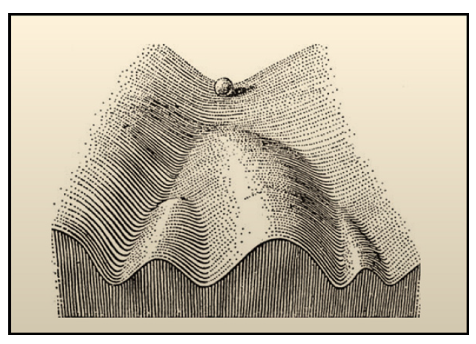
沃丁顿表观遗传景观(The Waddington's epigenetic landscape) 是描述基因调控下细胞分化的动态性的一个经典的隐喻，是由沃丁顿在1957年提出的。他将细胞分化比喻作从高处沿山坡滚落下的小球，直到一个稳定的盆地 (basin)，该盆地也就代表一定的分化状态。小球最开始能量较高，处于不稳定状态，对应干细胞等未分化的细胞状态，小球最终滚落于低能量的盆地，较稳定，对应分化后的细胞。小球（干细胞）沿着不同的路径最终可以进入不同的盆地（分化为不同的细胞）。图示如下：

 

 

接着介绍两篇数据驱动的建模 (建立landscape模型) 文章，两篇文章都是基于Artificial neural network中的Hopfield Network（HN）的，Artificial neural network也是构建基因调控网络的方法之一。第一篇基于离散的HN，第二篇基于连续的HN。

<Characterizing cancer subtypes as attractors of Hopfield networks [1]>

The GRN model of this paper is based on the artificial neural network, discretized Hopfield Network. In this paper, they use the static gene expression profiles to construct the discretized Hopfield Network to mapping cancer subtypes onto the attractors of the landscape.
Here’s a basic model of Hopfield Network:

 Each node represents a gene, and its output as the gene expression value, that is, state. The state of a node will be updated by all of its neighbors’ states within an iteration. The formula as follows:

 

 

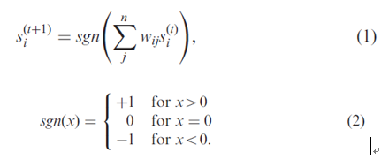
s_i(t) is the state of node i at time t, w_ij is the weight of the edge between node i and j.
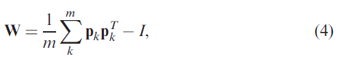
The W will be learned by Hebbian learning.

 

 

P is the pattern matrix, p=sgn(D), D is the expression matrix.
After several iterations, we can get a stable state. And the stable state can be visualized by the expression matrix.

 

 

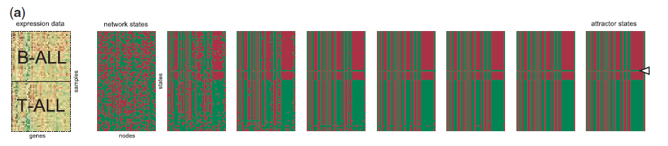
We can observe from the above figure that it gets into a stable state gradually, and the up and down parts corresponding to the subtype of cancer respectively, B-ALL and T-ALL. There is an error marked by a triangle in the upper stable state, but it won't influence the whole stable state.
Notably, they consider the sparse character of GRN, but the W learned by the Hebbian learning algorithm will be dense. They adopt a pruning method. At the premise of the accuracy of the classification of cells decrease within 20%, they delete the smaller weight edge.
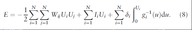
Then, to visualize the landscape, they use the PCA to reduce dimension. As regular, they divide mesh on the 2D plane and do inverse PCA to map mesh points into the high dimensional space. Finally, based on the mesh points and true data points, we use the energy function E to plot them in the 3-dimensional space.

E is a Lyapunov function.
Finally, by interpolating values, we can get the landscape with the surface.

 

<HopLand: single-cell pseudotime recovery using continuous Hopfield network-based modeling of Waddington’s epigenetic landscape  [2]>

The GRN model of this paper is based on the artificial neural network, Continuous Hopfield Network (CHN). In this paper, Hopland constructs landscape using continuous Hopfield Landscape (CHN) based on the gene expression data. And the pseudotime is estimated by the geodesic distance on the landscape. In this paper, they think the biological system cannot be characterized by the two-state discretized Hopfield Network, but a continuous relationship between input and output. As same as the last paper, each neuron represents a gene in the neural network.
As far as the model of CHN, v_i represents the output of neuron, namely, gene expression value, N is the gene number, the input of neuron consists of noise and other neurons' output. The change rate of neuron i can be modeled as:

 

 

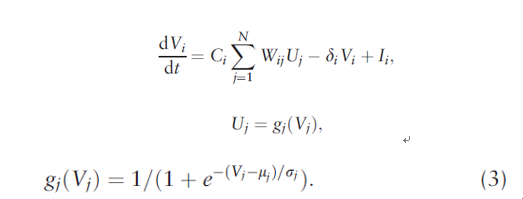
C_i is an amplifier, W_ij is the weight matrix, g_j() is the activated function, a sigmoid function as a g_j() here, it's monotone increasing to assure the stableness of system. δ_i is the degeneration rate of gene i, I_i is the outer input.
To inferred these parameters, they construct two objective functions to generate simulated data at the premise that a realistic model can generate simulated data consistent with the true data.

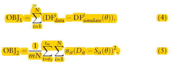
DF as the density function and the OBJ₁ to assure the distribution of true data and simulated data is consistent. And I can't understand OBJ₂ well.
A gradient descent learning algorithm is been used to update the parameters in the CHN.
The energy function here is also a Lyapunov function:

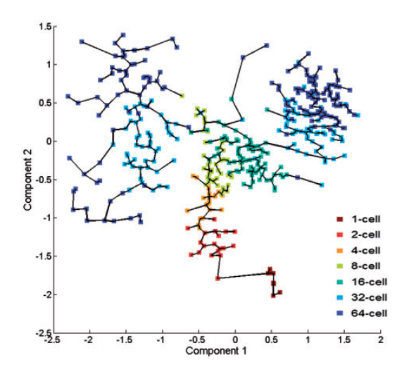
The steps of visualization of the landscape are consistent with the paper [1]. The only different point is the dimensionality reduction method, it uses nonlinear GP-LVM to replace the linear PCA. They think the nonlinear method is more suitable for biological information extraction.
To estimate the pseudotime, they use the fast marching algorithm to extract the geodesic distance and then construct the MST. The pseudotime of the i^th cell is estimated as the distance between the corresponding tree node with the root node.

 

Ref:

[1]. Maetschke S R, Ragan M A. Characterizing cancer subtypes as attractors of Hopfield networks[J]. Bioinformatics, 2014, 30(9): 1273-1279.
[2]. Guo J, Zheng J. HopLand: single-cell pseudotime recovery using continuous Hopfield network-based modeling of Waddington’s epigenetic landscape[J]. Bioinformatics, 2017, 33(14).