Understanding about numerical stability, convergence and consistency

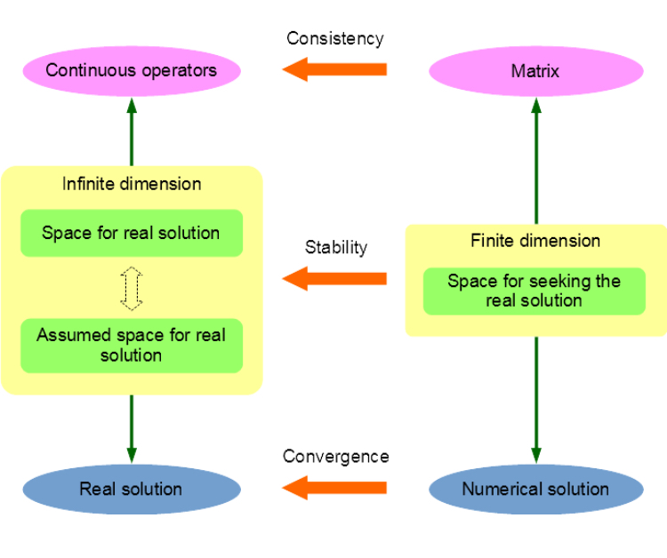
In a computer simulation of the real world, physical quantities, which usually have continuous distributions governed by partial differential equations (PDEs), can be solved by numerical methods such as finite element method (FEM) and boundary element method (BEM). Whether the obtained solution is a good approximation of the reality and whether the numerical schemes can proceed properly under perturbations of different error sources, such as numerical quadrature error and round-off error, should be clarified before any code implementation. To answer these questions, this post will introduce the fundamental concepts of numerical stability, convergence and consistency according to the following figure.

Let \(u\) be the real solution of the following general variational problem for a PDE:
\[
\text{Solve $u \in U$: } a(u, v) = (f, v) \quad (\forall v \in W),
\]
where both \(U\) and \(W\) are Hilbert spaces, \(a(\cdot, \cdot): U \times W \rightarrow \mathbb{K}\) with \(\mathbb{K} \in \{\mathbb{R}, \mathbb{C}\}\) is a sesquilinear or bilinear form and \(f: W \rightarrow \mathbb{K}\) is a continuous linear functional on \(W\). The solution \(u\) belongs to the space \(U\) of continuous functions with infinite dimension. For ease of further analysis, priori assumption is usually adopted for such function space thus we have the assumed function space \(V\). For example, the countably normed spaces \(V = B_{\varrho}(\Gamma)\) used in the \(hp\)-BEM is defined as
\[
B_{\varrho}(\Gamma) = \{ v \in L^2(\Gamma): v \circ \kappa_K \in B_{\varrho}(K_0) \},
\]
where

• \(\Gamma\) is the boundary manifold of the solution domain, which is covered by the mesh \(\{K_i\}_{i=1}^{N_M}\) with \(N_M\) as the number of mesh elements;
• \(K_0\) is the reference cell and \(K\) is the real cell which may be curved;
• \(\kappa_K: K_0 \rightarrow K\) is the mapping from the reference cell to the real cell;
• \(B_{\varrho}(K_0)\) is the countably normed space restricted on the reference cell, which has constraints on the norm of all the derivatives of \(v\). Its formulation is given as below: \[ B_{\varrho}(K_0) = \big\{ v \in L^2(K_0): \Norm{r_X^{k - \varrho} \left( \Pd{}{r_X} \right)^k \left( \vartheta (\alpha_X - \vartheta_X) \right)^{l - \varrho} \left( \Pd{}{\vartheta_X} \right)^l v}_{L^2(U_X)} \leq C d^{k+l+1} k! l!\big\}, \] for which I do not provide more explanation in this post, but just give you an impression that the construction of the assumed solution function space can be quite complicated.

To solve the PDE on a computer, a finite dimensional subspace \(V^L\) of \(V\) must be constructed, in which a solution is to be sought as an approximation of the real solution by using some sort of numerical method. Then the stability condition means, for any function \(u\) in the real space \(U\) or the assumed space \(V\) of infinite dimension, whether there exists a function \(v\) in the finite dimensional space \(V^L\), such that the norm of their difference can be controlled to be arbitrarily small as \(N_L\), the dimension of space \(V^L\), increases. For example, in the \(hp\)-BEM, a subspace \(V^L\) can be constructed to have the following exponential stability condition:
\[
\begin{equation}
\label{eq:stability-condition}
\forall u \in B_{\varrho}(\Gamma): \inf_{v \in V^L} \norm{u - v}_{L^2(\Gamma)} \leq C \exp(-b N_L^{1/4}).
\end{equation}
\]

Once the solution \(u^L \in V^L\) for the finite dimensional problem is obtained from a general method such as the Galerkin method, i.e.
\[
\text{Solve $u^L \in V^L$: } a(u^L, v) = (f, v) \quad (\forall v \in V^L),
\]
the concept of convergence comes into play, which ensures that the difference between this \(u^L\) and the real solution \(u\) can be controlled. For example, if the following condition can be satisfied:
\[
\Norm{P_L A u^L} \geq C_s \Norm{u^L} \quad (\forall u^L \in V^L),
\]
where \(P_L: V \rightarrow V^L\) is the projection operator, \(A: V^L \rightarrow (V^L)'\) is the associated operator of the sesquilinear or bilinear form \(a(\cdot, \cdot)\) and \(C_s > 0\) is a constant, it can be proved that the solution obtained from the Galerkin method satisfies
\[
\begin{equation}
\label{eq:convergence-condition}
\norm{u - u^L} \leq C \inf_{v \in V^L} \Norm{u - v}.
\end{equation}
\]
This means the real solution can be properly approximated by the Galerkin solution with the error norm controlled by the approximation capability of the adopted finite dimensional space \(V^L\), and we say the method is convergent. In addition, combing equation \eqref{eq:stability-condition} and \eqref{eq:convergence-condition}, we know the solution has the exponential convergence property:
\[
\begin{equation}
\label{eq:exponential-convergence}
\norm{u - u^L} \leq C \exp(-b N_L^{1/4}).
\end{equation}
\]

Finally, we introduce the concept of consistency. During the discretization of the problem, the sesquilinear or bilinear form \(a(\cdot, \cdot)\), or rather, its associated operator \(A\), is to be approximated by its discrete version, i.e. the stiffness matrix \(A^L\). The evaluation of \(A^L\)'s coefficients usually needs numerical quadrature techniques, which introduces additional numerical error. Even though there is an analytical formula for integration, round-off error limited by the finite computer byte length is unavoidable. Hence, an operator \(\tilde{A}^L\) is obtained being different from \(A^L\). The error between \(A^L\) and \(\tilde{A}^L\) will perturb the adopted numerical method. If the error between the real and numerical solutions \(\Norm{u - \tilde{u}^L}\) can still be controlled, we say the method is consistent. For example, in the \(hp\)-BEM, if the stiffness matrix coefficient error satisfies the following consistent condition
\[
\abs{A^L_{ij} - \tilde{A}^L_{ij}} < \Phi(L) \quad (i,j = 1, \cdots, N_L)
\]
with
\[
\lim_{L \rightarrow \infty} N_L \Phi(L) = 0 \; \text{and} \; \Phi(L) = N_L^{-1} L \sigma^{\varrho L},
\]
the exponential convergence as shown in \eqref{eq:exponential-convergence} can be preserved.