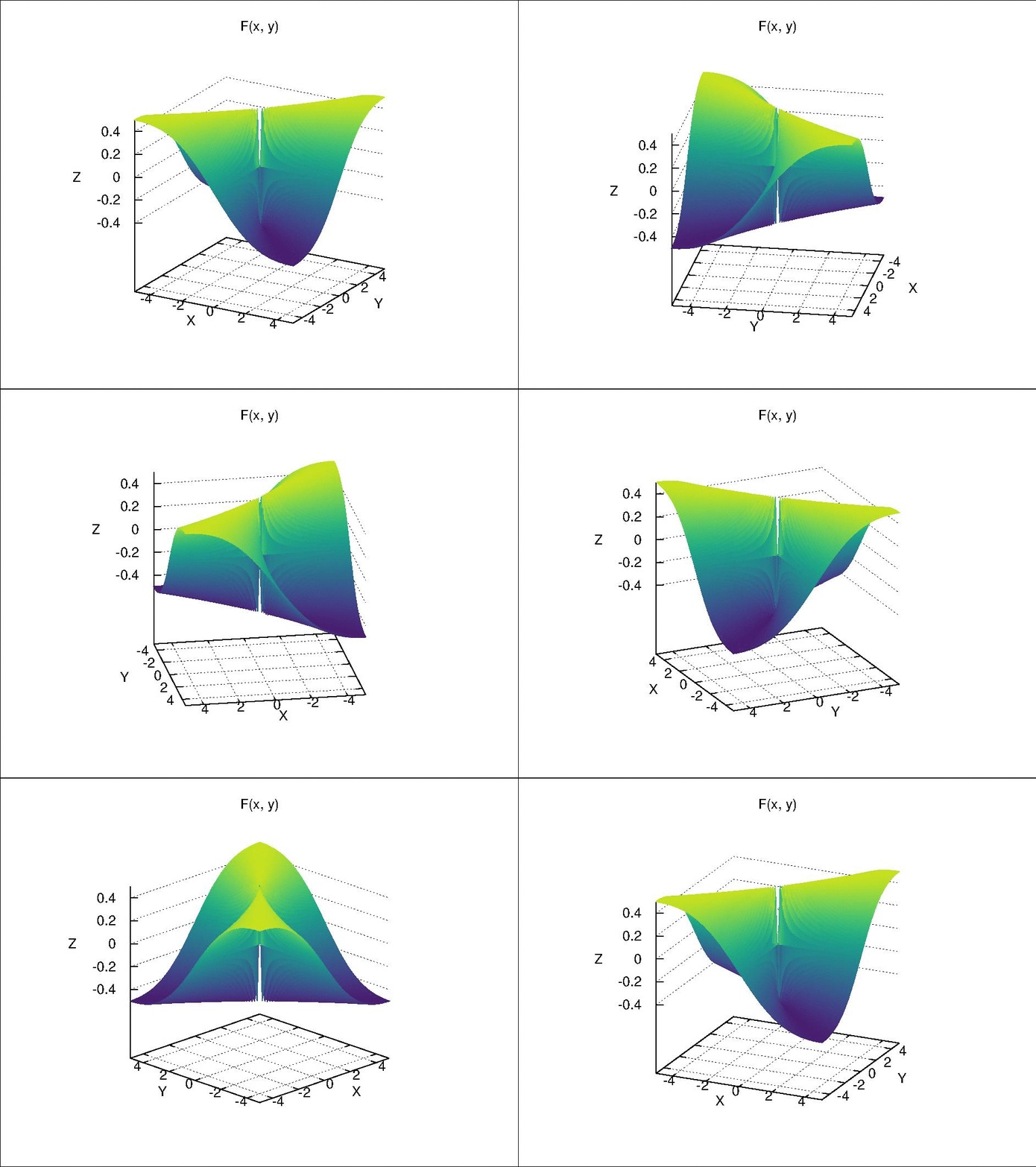
James Munkres Topology: Sec 18 Exer 12
Theorem 18.4 in James Munkres “Topology” states that if a function \(f : A \rightarrow X \times Y\) is continuous, its coordinate functions \(f_1 : A \rightarrow X\) and \(f_2 : A \rightarrow Y\) are also continuous, and the converse is also true. This is what we have been familiar with, such as a continuous parametric curve \(f: [0, 1] \rightarrow \mathbb{R}^3\) defined as \(f(t) = (x(t), y(t), z(t))^T\) with its three components being continuous. However, if a function \(g: A \times B \rightarrow X\) is separately continuous in each of its components, i.e. both \(g_1: A \rightarrow X\) and \(g_2 : B \rightarrow X\) are continuous, \(g\) is not necessarily continuous.
Here, the said “separately continuous in each of its components” means arbitrarily selecting the value of one component variable from its domain and fix it, then the original function depending only on the other component is continuous. In the above, the function \(g\) can be envisaged as a curved surface in 3D space. With \(g_1\) being continuous, the intersection profiles between this curved surface and those planes perpendicular to the coordinate axis for \(B\) are continuous. Similarly, because \(g_2\) is continuous, the intersection profiles obtained from those planes perpendicular to the coordinate axis for \(A\) are also continuous. The continuity of intersection curves is only ensured in these two special directions, so it is not guaranteed that the original function \(g\) is continuous.
In Exercise 12 of Section 18, an example is given as
\[
F(x \times y) = \begin{cases}
\frac{xy}{x^2 + y^2} & (x \neq 0, y \neq 0) \\
0 & (x = 0, y = 0)
\end{cases},
\]
where \(F\) is continuous separately in each of its component variables but is not continuous by itself. This is function is visualized below.

Fix \(y\) at \(y_0\), we have \(F_{y_0}(x) = F(x \times y_0)\). When \(y_0 \neq 0\), \(F_{y_0}(x)\) is continuous with respect to \(x\) because it is only a composition of continuous real valued functions via simple arithmetic. When \(y_0 = 0\), if \(x \neq 0\), \(F_0(x) = 0\); if \(x =0\), \(F_0(x)\) is also 0 due to the definition of \(F(x \times y)\). Therefore, \(F_0(x)\) is a constant function, which is continuous due to Theorem 18.2 (a). Similarly, \(F_{x_0}(y)\) is also continuous with respect to \(y\).
However, if we let \(x = y\) and approach \((x, y) = (x, x)\) to \((0, 0)\), it can be seen that \(F(x \times x)\) is not continuous, because
- when \(x \neq 0\), \(F(x \times x) = \frac{x^2}{x^2 + x^2} = \frac{1}{2}\);
- when \(x = 0\), \(F(x \times x) = 0\).
If we let \(x = -y\) and approach \((x ,y) = (x, -x)\) to \((0, 0)\), \(F = -\frac{1}{2}\) when \(x \neq 0\) and \(F = 0\) when \(x = 0\).
Then, if we select an open set such as \((-\frac{1}{4}, \frac{1}{4})\) around the function value \(0\) in \(\mathbb{R}\), its pre-image \(U\) in \(\mathbb{R} \times \mathbb{R}\) should include the point \((0, 0)\) and exclude the rays \((x, x)\) and \((x, -x)\) with \(x \in \mathbb{R}\) and \(x \neq 0\). Due to these excluded rays, there is no neighborhood of \((0, 0)\) in \(\mathbb{R} \times \mathbb{R}\) that is contained completely in \(U\). Therefore, \(U\) is not an open set and \(F(x \times y)\) is not continuous.
From the above analysis, some lessons can be learned.
- Pure analysis can be made and general conclusions can be obtained before entering into the real world with a solid example.
- A tangible counter example is a sound proof for negation of a proposition. Just one is enough!


 浙公网安备 33010602011771号