Web Scraping and Applied Clustering Global Happiness and Social Progress Index
Increasing amount of data is available on the web. Web scraping is a technique developed to extract data from web pages automatically and transforming it into a data format for further data analysis and insights. Applied clustering is an unsupervised learning technique that refers to a family of pattern discovery and data mining tools with applications in machine learning, bioinformatics, image analysis, and segmentation of consumer types, among others. R offers several packages and tools for web scraping, data manipulation, statistical analysis and machine learning. The motivation for this post is to illustrate the applications of web scraping, dimension reduction and applied clustering tools in R.
There are two separate data sets for web scraping in this post. The first data set is from a recently released World Happiness Report 2017 by the United Nations Sustainable Development Solutions Network. The 2017 report launched on March 20, the day of world happiness, contained global rankings for happiness and social well-being. The second data set for web scraping is the 2015 social progress index of countries in the world. Social Progress Index has been described as measuring the extent to which countries provide for the social and environmental needs of their citizens. In this exercise, the two data sets joined by country column were pre-processed prior to principal component analysis (PCA) and clustering. The goals of the clustering approach in this post were to segment rows of the over 150 countries in the data into separate groups (clusters), The expectation is that sets of countries within a cluster are as similar as possible to each other for happiness and social progress, and as dissimilar as possible to the other sets of countries assigned in different clusters.
Load Required Packages
require(rvest)
require(magrittr)
require(plyr)
require(dplyr)
require(reshape2)
require(ggplot2)
require(FactoMineR)
require(factoextra)
require(cluster)
require(useful)
Web Scraping and Data Pre-processing
# Import the first data set from the site
url1 <- "https://en.wikipedia.org/wiki/World_Happiness_Report"
happy %
        html_nodes("table") %>%
        extract2(1) %>%
        html_table()

# inspect imported data structure

str(happy)
## 'data.frame':    155 obs. of  12 variables:
##  $ Overall Rank                : int  1 2 3 4 5 6 7 8 9 10 ...
##  $ Change in rank              : int  3 -1 0 -2 0 1 -1 0 0 0 ...
##  $ Country                     : chr  "Norway" "Denmark" "Iceland" "Switzerland" ...
##  $ Score                       : num  7.54 7.52 7.5 7.49 7.47 ...
##  $ Change in score             : num  0.039 -0.004 0.003 -0.015 0.056 0.038 -0.088 -0.02 -0.029 -0.007 ...
##  $ GDP per capita              : num  1.62 1.48 1.48 1.56 1.44 ...
##  $ Social support              : num  1.53 1.55 1.61 1.52 1.54 ...
##  $ Healthy life expectancy     : num  0.797 0.793 0.834 0.858 0.809 0.811 0.835 0.817 0.844 0.831 ...
##  $ Freedom to make life choices: num  0.635 0.626 0.627 0.62 0.618 0.585 0.611 0.614 0.602 0.613 ...
##  $ Generosity                  : num  0.362 0.355 0.476 0.291 0.245 0.47 0.436 0.5 0.478 0.385 ...
##  $ Trust                       : num  0.316 0.401 0.154 0.367 0.383 0.283 0.287 0.383 0.301 0.384 ...
##  $ Dystopia                    : num  2.28 2.31 2.32 2.28 2.43 ...
Pre-process the first data set for analysis:
## Exclude columns with ranks and scores, retain the other columns
happy <- happy[c(3,6:11)]
### rename column headers
colnames(happy) <- gsub(" ", "_", colnames(happy), perl=TRUE)
names(happy)
## [1] "Country"                      "GDP_per_capita"
## [3] "Social_support"               "Healthy_life_expectancy"
## [5] "Freedom_to_make_life_choices" "Generosity"
## [7] "Trust"
### standardize names of selected countries to confirm with country names in the the map database
happy$Country <- as.character(mapvalues(happy$Country,
                                        from = c("United States", "Congo (Kinshasa)", "Congo (Brazzaville)", "Trinidad and Tobago"),
                                        to = c("USA","Democratic Republic of the Congo", "Democratic Republic of the Congo", "Trinidad")))
Import the second data set from the web
### scrape social progress index data report from the site
url2 <- "https://en.wikipedia.org/wiki/List_of_countries_by_Social_Progress_Index"
social %
     html_nodes("table") %>%
     .[[2]] %>%
     html_table(fill=T)
# check imported data structure
str(social)
## 'data.frame':    163 obs. of  9 variables:
##  $ Country                  : chr  "Norway" "Sweden" "Switzerland" "Iceland" ...
##  $ Rank (SPI)               : chr  "1" "2" "3" "4" ...
##  $ Social Progress Index    : chr  "88.36" "88.06" "87.97" "87.62" ...
##  $ Rank (BHN)               : chr  "9" "8" "2" "6" ...
##  $ Basic Human Needs        : chr  "94.8" "94.83" "95.66" "95" ...
##  $ Rank (FW)                : chr  "1" "3" "2" "4" ...
##  $ Foundations of Well-being: chr  "88.46" "86.43" "86.5" "86.11" ...
##  $ Rank (O)                 : chr  "9" "5" "10" "11" ...
##  $ Opportunity              : chr  "81.82" "82.93" "81.75" "81.73" ...
Pre-process the second data set for analysis:
### Again, exclude columns with ranks, keep the rest
social <- social[c(1,5,7,9)]
### rename column headers
names(social) <- c("Country", "basic_human_needs", "foundations_well_being", "opportunity")

### Standardize country names to confirm with country names in the map dataset
social$Country <- as.character(mapvalues(social$Country,
                                         from = c("United States", "Côte d'Ivoire","Democratic Republic of Congo", "Congo", "Trinidad and Tobago"),
                                         to=c("USA", "Ivory Cost","Democratic Republic of the Congo", "Democratic Republic of the Congo", "Trinidad")))

## coerce character data columns to numeric
social[, 2:4] <- sapply(social[, 2:4], as.numeric)
## Warning in lapply(X = X, FUN = FUN, ...): NAs introduced by coercion
## Warning in lapply(X = X, FUN = FUN, ...): NAs introduced by coercion
## Warning in lapply(X = X, FUN = FUN, ...): NAs introduced by coercion
Join the two imported data sets
### perform left join
soc.happy <- left_join(happy, social, by = c('Country' = 'Country'))
### check for missing values in the combined data set
mean(is.na(soc.happy[, 2:10]))
## [1] 0.0353857
Left joining the two data files introduced missing values (approximately 3.5% of the total data set) in the combined data set. R offers a variety of imputation algorithms to populate missing values. In this post, a median imputation strategy was applied by replacing missing values with the median for each column.
### median imputation
for(i in 1:ncol(soc.happy[, 2:10])) {
        soc.happy[, 2:10][is.na(soc.happy[, 2:10][,i]), i] <- median(soc.happy[, 2:10][,i], na.rm = TRUE)
}
### summary of the raw data
summary(soc.happy[,2:10])
##  GDP_per_capita   Social_support  Healthy_life_expectancy
##  Min.   :0.0000   Min.   :0.000   Min.   :0.0000
##  1st Qu.:0.6600   1st Qu.:1.042   1st Qu.:0.3570
##  Median :1.0550   Median :1.252   Median :0.6050
##  Mean   :0.9779   Mean   :1.187   Mean   :0.5474
##  3rd Qu.:1.3150   3rd Qu.:1.412   3rd Qu.:0.7190
##  Max.   :1.8710   Max.   :1.611   Max.   :0.9490
##  Freedom_to_make_life_choices   Generosity         Trust
##  Min.   :0.0000               Min.   :0.0000   Min.   :0.0000
##  1st Qu.:0.3010               1st Qu.:0.1530   1st Qu.:0.0570
##  Median :0.4370               Median :0.2320   Median :0.0890
##  Mean   :0.4078               Mean   :0.2461   Mean   :0.1224
##  3rd Qu.:0.5140               3rd Qu.:0.3220   3rd Qu.:0.1530
##  Max.   :0.6580               Max.   :0.8380   Max.   :0.4640
##  basic_human_needs foundations_well_being  opportunity
##  Min.   :26.81     Min.   :44.12          Min.   :21.12
##  1st Qu.:61.94     1st Qu.:63.09          1st Qu.:41.43
##  Median :75.73     Median :69.41          Median :49.55
##  Mean   :71.82     Mean   :68.29          Mean   :52.12
##  3rd Qu.:84.73     3rd Qu.:74.79          3rd Qu.:62.83
##  Max.   :96.03     Max.   :88.46          Max.   :86.58
An important procedure for meaningful clustering and dimension reduction steps involves data transformation and scaling variables. The simple function below will transform all variables to values between 0 and 1.
## transform variables to a range of 0 to 1
range_transform <- function(x) {
     (x - min(x))/(max(x)-min(x))
 }
soc.happy[,2:10] <- as.data.frame(apply(soc.happy[,2:10], 2, range_transform))

### summary of transformed data shows success of transformation
summary(soc.happy[,2:10])
##  GDP_per_capita   Social_support   Healthy_life_expectancy
##  Min.   :0.0000   Min.   :0.0000   Min.   :0.0000
##  1st Qu.:0.3528   1st Qu.:0.6468   1st Qu.:0.3762
##  Median :0.5639   Median :0.7772   Median :0.6375
##  Mean   :0.5227   Mean   :0.7367   Mean   :0.5768
##  3rd Qu.:0.7028   3rd Qu.:0.8765   3rd Qu.:0.7576
##  Max.   :1.0000   Max.   :1.0000   Max.   :1.0000
##  Freedom_to_make_life_choices   Generosity         Trust
##  Min.   :0.0000               Min.   :0.0000   Min.   :0.0000
##  1st Qu.:0.4574               1st Qu.:0.1826   1st Qu.:0.1228
##  Median :0.6641               Median :0.2768   Median :0.1918
##  Mean   :0.6198               Mean   :0.2936   Mean   :0.2638
##  3rd Qu.:0.7812               3rd Qu.:0.3842   3rd Qu.:0.3297
##  Max.   :1.0000               Max.   :1.0000   Max.   :1.0000
##  basic_human_needs foundations_well_being  opportunity
##  Min.   :0.0000    Min.   :0.0000         Min.   :0.0000
##  1st Qu.:0.5075    1st Qu.:0.4278         1st Qu.:0.3103
##  Median :0.7067    Median :0.5704         Median :0.4343
##  Mean   :0.6503    Mean   :0.5451         Mean   :0.4735
##  3rd Qu.:0.8368    3rd Qu.:0.6917         3rd Qu.:0.6372
##  Max.   :1.0000    Max.   :1.0000         Max.   :1.0000
Although the previous data transformation step could have been adequate for next steps of this analysis, the function shown below would re-scale all variables to a mean of 0 and standard deviation of 1.
## Scaling variables to a mean of 0 and standard deviation of 1
sd_scale <- function(x) {
     (x - mean(x))/sd(x)
 }
soc.happy[,2:10] <- as.data.frame(apply(soc.happy[,2:10], 2, sd_scale))

### summary of the scaled data
summary(soc.happy[,2:10])
##  GDP_per_capita    Social_support    Healthy_life_expectancy
##  Min.   :-2.3045   Min.   :-4.1377   Min.   :-2.2984
##  1st Qu.:-0.7492   1st Qu.:-0.5050   1st Qu.:-0.7994
##  Median : 0.1817   Median : 0.2271   Median : 0.2419
##  Mean   : 0.0000   Mean   : 0.0000   Mean   : 0.0000
##  3rd Qu.: 0.7944   3rd Qu.: 0.7849   3rd Qu.: 0.7206
##  Max.   : 2.1046   Max.   : 1.4787   Max.   : 1.6863
##  Freedom_to_make_life_choices   Generosity          Trust
##  Min.   :-2.7245              Min.   :-1.8320   Min.   :-1.2102
##  1st Qu.:-0.7137              1st Qu.:-0.6929   1st Qu.:-0.6467
##  Median : 0.1949              Median :-0.1048   Median :-0.3304
##  Mean   : 0.0000              Mean   : 0.0000   Mean   : 0.0000
##  3rd Qu.: 0.7093              3rd Qu.: 0.5652   3rd Qu.: 0.3023
##  Max.   : 1.6713              Max.   : 4.4067   Max.   : 3.3767
##  basic_human_needs foundations_well_being  opportunity
##  Min.   :-2.6059   Min.   :-2.5434        Min.   :-1.9025
##  1st Qu.:-0.5721   1st Qu.:-0.5471        1st Qu.:-0.6559
##  Median : 0.2263   Median : 0.1180        Median :-0.1575
##  Mean   : 0.0000   Mean   : 0.0000        Mean   : 0.0000
##  3rd Qu.: 0.7474   3rd Qu.: 0.6842        3rd Qu.: 0.6576
##  Max.   : 1.4016   Max.   : 2.1228        Max.   : 2.1154
Simple correlation analysis
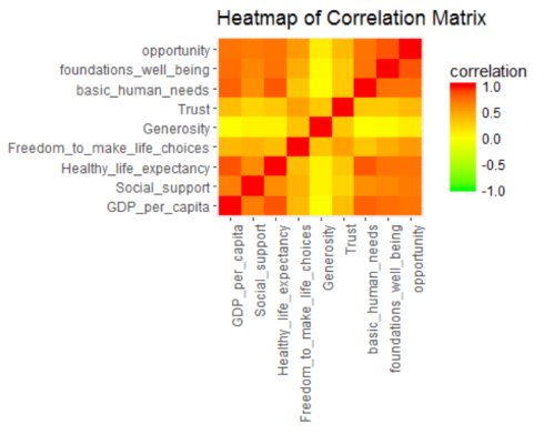
Now, the data is ready to explore variable relationships with each other.
corr <- cor(soc.happy[, 2:10], method="pearson")
ggplot(melt(corr, varnames=c("x", "y"), value.name="correlation"),
       aes(x=x, y=y)) +
             geom_tile(aes(fill=correlation)) +
             scale_fill_gradient2(low="green", mid="yellow", high="red",
             guide=guide_colorbar(ticks=FALSE, barheight = 5),
             limits=c(-1,1)) +
             theme(axis.text.x = element_text(angle = 90, hjust = 1)) +
             labs(title="Heatmap of Correlation Matrix",
                  x=NULL, y=NULL)
Principal Component Analysis
Principal component analysis is a multivariate statistics widely used for examining relationships among several quantitative variables. PCA identifies patterns in the variables to reduce the dimensions of the data set in multiple regression and clustering, among others.
soc.pca <- PCA(soc.happy[, 2:10], graph=FALSE)
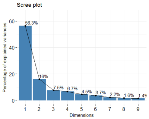
fviz_screeplot(soc.pca, addlabels = TRUE, ylim = c(0, 65))
The percentages on each bar indicate the proportion of total variance explained by the respective principal component. As seen in the scree plot, the first three principal components accounted for ~80% of the total variance.
soc.pca$eig
##        eigenvalue percentage of variance cumulative percentage of variance
## comp 1  5.0714898              56.349887                          56.34989
## comp 2  1.4357885              15.953205                          72.30309
## comp 3  0.6786121               7.540134                          79.84323
## comp 4  0.6022997               6.692219                          86.53544
## comp 5  0.4007136               4.452373                          90.98782
## comp 6  0.3362642               3.736269                          94.72409
## comp 7  0.2011131               2.234590                          96.95868
## comp 8  0.1471443               1.634937                          98.59361
## comp 9  0.1265747               1.406386                         100.00000
The output suggests that the first two principal components are worthy of consideration. A practical guide to determining the optimum number of principal component axes could be to consider only those components with eigen values greater than or equal to 1.
# Contributions of variables to principal components
soc.pca$var$contrib[,1:3]
##                                   Dim.1        Dim.2        Dim.3
## GDP_per_capita               15.7263477 2.455323e+00 3.162470e-02
## Social_support               12.0654754 5.445993e-01 1.345610e+00
## Healthy_life_expectancy      15.1886385 2.259270e+00 3.317633e+00
## Freedom_to_make_life_choices  6.6999181 2.207049e+01 8.064596e+00
## Generosity                    0.3270114 4.189437e+01 5.406678e+01
## Trust                         4.3688692 2.570658e+01 3.211058e+01
## basic_human_needs            14.5402807 3.836956e+00 1.021076e+00
## foundations_well_being       15.1664220 1.232353e+00 4.169125e-02
## opportunity                  15.9170370 6.170376e-05 4.113192e-04
The first principal component explained approximately 57% of the total variation and appears to represent opportunity, GDP per capita, healthy life expectancy, Foundations of Well-being, and basic human needs.
The second principal component explained a further 16% of the total variation and represented opportunity, social support, and generosity.
Applied Clustering
The syntax for clustering algorithms require specifying the number of desired clusters (k=) as an input. The practical issue is what value should k take? In the absence of a subject-matter knowledge, R offers various empirical approaches for selecting a value of k. One such R tool for suggested best number of clusters is the NbClust package.
require(NbClust)
nbc <- NbClust(soc.happy[, 2:10], distance="manhattan",
               min.nc=2, max.nc=30, method="ward.D", index='all')
## Warning in pf(beale, pp, df2): NaNs produced
## *** : The Hubert index is a graphical method of determining the number of clusters.
##                 In the plot of Hubert index, we seek a significant knee that corresponds to a
##                 significant increase of the value of the measure i.e the significant peak in Hubert
##                 index second differences plot.
##

## *** : The D index is a graphical method of determining the number of clusters.
##                 In the plot of D index, we seek a significant knee (the significant peak in Dindex
##                 second differences plot) that corresponds to a significant increase of the value of
##                 the measure.
##
## *******************************************************************
## * Among all indices:
## * 4 proposed 2 as the best number of clusters
## * 9 proposed 3 as the best number of clusters
## * 3 proposed 4 as the best number of clusters
## * 1 proposed 5 as the best number of clusters
## * 1 proposed 9 as the best number of clusters
## * 1 proposed 16 as the best number of clusters
## * 1 proposed 28 as the best number of clusters
## * 2 proposed 29 as the best number of clusters
## * 1 proposed 30 as the best number of clusters
##
##                    ***** Conclusion *****
##
## * According to the majority rule, the best number of clusters is  3
##
##
## *******************************************************************
The NbClust algorithm suggested a 3-cluster solution to the combined data set. So, we will apply K=3 in next steps.
set.seed(4653)
pamK3 <- pam(soc.happy[, 2:10], diss=FALSE, 3, keep.data=TRUE)
# Number of countries assigned in the three clusters
fviz_silhouette(pamK3)
##   cluster size ave.sil.width
## 1       1   28          0.40
## 2       2   82          0.29
## 3       3   47          0.27
The number of countries assigned in each cluster is displayed in the table above.
An interesting aspect of the K-medoids algorithm is that it finds observations from the data that are typical of each cluster. So, the following code will ask for a list of “the typical countries” as selected by the algorithm to be closest to the center of the cluster.
## which countries were typical of each cluster
soc.happy$Country[pamK3$id.med]
## [1] "Germany"      "Macedonia"    "Burkina Faso"
Putting it together
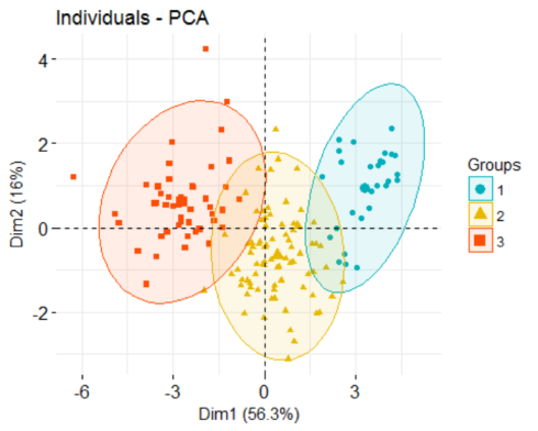
We can now display individual countries and superimpose their cluster assignments on the plane defined by the first two principal components.
soc.happy['cluster'] <- as.factor(pamK3$clustering)

fviz_pca_ind(soc.pca,
             label="none",
             habillage = soc.happy$cluster, #color by cluster
             palette = c("#00AFBB", "#E7B800", "#FC4E07", "#7CAE00", "#C77CFF", "#00BFC4"),
             addEllipses=TRUE
)
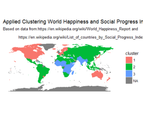
Finally, displaying clusters of countries on a world map
map.world <- map_data("world")
# LEFT JOIN
map.world_joined <- left_join(map.world, soc.happy, by = c('region' = 'Country'))
ggplot() +
        geom_polygon(data = map.world_joined, aes(x = long, y = lat, group = group, fill=cluster, color=cluster)) +
        labs(title = "Applied Clustering World Happiness and Social Progress Index",
             subtitle = "Based on data from:https://en.wikipedia.org/wiki/World_Happiness_Report and\n
             https://en.wikipedia.org/wiki/List_of_countries_by_Social_Progress_Index",
             x=NULL, y=NULL) +
        coord_equal() +
        theme(panel.grid.major=element_blank(),
              panel.grid.minor=element_blank(),
              axis.text.x=element_blank(),
              axis.text.y=element_blank(),
              axis.ticks=element_blank(),
              panel.background=element_blank()
        )
Concluding Remarks
Cluster analysis and dimension reduction algorithms such as PCA are widely used approaches to split data sets into distinct subsets of groups as well as to reduce the dimensionality of the variables, respectively. Together, these analytics approaches: 1) make the structure of the data easier to understand, and 2) also make subsequent data mining tasks easier to perform. Hopefully, this post has attempted to illustrate the applications of web scraping, pre-processing data for analysis, PCA, and cluster analysis using various tools available in R. Please let us know your comments and suggestions. Ok to networking with the author in LinkdIn.
转自:https://datascienceplus.com/web-scraping-and-applied-clustering-global-happiness-and-social-progress-index/


 浙公网安备 33010602011771号