机器学习工程师 - Udacity 使用特征脸方法和 SVM 进行脸部识别

在此示例中使用的数据集来自“Labeled Faces in the Wild”，亦称为 LFW_ Download (233MB) 并经过预处理。这是原始数据。

from time import time
import logging
import pylab as pl
import numpy as np
​
from sklearn.model_selection import train_test_split
from sklearn.datasets import fetch_lfw_people
from sklearn.model_selection import GridSearchCV
from sklearn.metrics import classification_report
from sklearn.metrics import confusion_matrix
from sklearn.decomposition import RandomizedPCA
from sklearn.decomposition import PCA
from sklearn.svm import SVC

 

加载数据集

# Download the data, if not already on disk and load it as numpy arrays
lfw_people = fetch_lfw_people('data', min_faces_per_person=70, resize=0.4)
​
# introspect the images arrays to find the shapes (for plotting)
n_samples, h, w = lfw_people.images.shape
np.random.seed(42)
​
​
# for machine learning we use the data directly (as relative pixel
# position info is ignored by this model)
X = lfw_people.data
n_features = X.shape[1]
​
# the label to predict is the id of the person
y = lfw_people.target
target_names = lfw_people.target_names
n_classes = target_names.shape[0]
​
print("Total dataset size:")
print("n_samples: %d" % n_samples)
print("n_features: %d" % n_features)
print( "n_classes: %d" % n_classes)

Total dataset size:
n_samples: 1288
n_features: 1850
n_classes: 7

拆分为训练集和测试集

X_train, X_test, y_train, y_test = train_test_split(X, y, test_size=0.25, random_state=42)

 

计算 PCA
我们现在可以对脸部数据集（当做无标签数据集）计算 PCA（特征脸）了：无监督式特征提取/降维。

n_components = 150
​
print( "Extracting the top %d eigenfaces from %d faces" % (n_components, X_train.shape[0]) )
t0 = time()
​
# TODO: Create an instance of PCA, initializing with n_components=n_components and whiten=True
pca = PCA(n_components=n_components, whiten=True, svd_solver='randomized')
​
#TODO: pass the training dataset (X_train) to pca's 'fit()' method
pca = pca.fit(X_train)
print("done in %0.3fs" % (time() - t0))

Extracting the top 150 eigenfaces from 966 faces
done in 0.349s

将输入数据投射到特征脸标准正交基

eigenfaces = pca.components_.reshape((n_components, h, w))
​
t0 = time()
X_train_pca = pca.transform(X_train)
X_test_pca = pca.transform(X_test)
print("done in %0.3fs" % (time() - t0))

done in 0.034s

​
训练 SVM 分类模型
我们将 SVM 分类器拟合到训练集中。我们将使用 GridSearchCV 为该分类器找到一组合适的参数。

param_grid = {
'C': [1e3, 5e3, 1e4, 5e4, 1e5],
'gamma': [0.0001, 0.0005, 0.001, 0.005, 0.01, 0.1],
}
​
# for sklearn version 0.16 or prior, the class_weight parameter value is 'auto'
clf = GridSearchCV(SVC(kernel='rbf', class_weight='balanced'), param_grid)
clf = clf.fit(X_train_pca, y_train)
​
print("Best estimator found by grid search:")
print(clf.best_estimator_)

Best estimator found by grid search:
SVC(C=1000.0, cache_size=200, class_weight='balanced', coef0=0.0,
  decision_function_shape='ovr', degree=3, gamma=0.001, kernel='rbf',
  max_iter=-1, probability=False, random_state=None, shrinking=True,
  tol=0.001, verbose=False)

用测试集评估模型质量

1. 分类报告
训练好分类器后，我们在测试数据集上运行该分类器，并定性地评估结果。Sklearn 的分类报告显示了每个类别的一些主要分类指标。

y_pred = clf.predict(X_test_pca)
​
print(classification_report(y_test, y_pred, target_names=target_names))

                   precision    recall  f1-score   support

     Ariel Sharon       0.56      0.69      0.62        13
     Colin Powell       0.74      0.87      0.80        60
  Donald Rumsfeld       0.76      0.81      0.79        27
    George W Bush       0.93      0.87      0.90       146
Gerhard Schroeder       0.76      0.76      0.76        25
      Hugo Chavez       0.73      0.53      0.62        15
       Tony Blair       0.88      0.83      0.86        36

      avg / total       0.84      0.83      0.83       322

2. 混淆矩阵
查看分类器效果的另一种方式是查看混淆矩阵。为此，我们可以直接调用 sklearn.metrics.confusion_matrix：

print(confusion_matrix(y_test, y_pred, labels=range(n_classes)))

[[  9   0   3   1   0   0   0]
 [  2  52   1   4   0   1   0]
 [  4   0  22   1   0   0   0]
 [  1  11   2 127   3   1   1]
 [  0   2   0   1  19   1   2]
 [  0   3   0   1   2   8   1]
 [  0   2   1   2   1   0  30]]

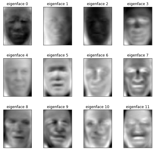
3. 绘制最显著的特征脸

def plot_gallery(images, titles, h, w, n_row=3, n_col=4):
"""Helper function to plot a gallery of portraits"""
pl.figure(figsize=(1.8 * n_col, 2.4 * n_row))
pl.subplots_adjust(bottom=0, left=.01, right=.99, top=.90, hspace=.35)
for i in range(n_row * n_col):
pl.subplot(n_row, n_col, i + 1)
pl.imshow(images[i].reshape((h, w)), cmap=pl.cm.gray)
pl.title(titles[i], size=12)
pl.xticks(())
pl.yticks(())
​
​
​
# plot the result of the prediction on a portion of the test set
​
def title(y_pred, y_test, target_names, i):
pred_name = target_names[y_pred[i]].rsplit(' ', 1)[-1]
true_name = target_names[y_test[i]].rsplit(' ', 1)[-1]
return ('predicted: %s\ntrue: %s' % (pred_name, true_name))
​
prediction_titles = [title(y_pred, y_test, target_names, i)
for i in range(y_pred.shape[0])]
​
plot_gallery(X_test, prediction_titles, h, w)
​
pl.show()

eigenface_titles = ["eigenface %d" % i for i in range(eigenfaces.shape[0])]
plot_gallery(eigenfaces, eigenface_titles, h, w)
​
pl.show()