回归算法、分类算法的损失函数的图示

 

 

 

 

 

 

 

?

1 2 3 4 5 6 7 8 9 10 11 12 13 14 15 16 17 18 19 20 21 22 23 24 25 26 27 28 29 30 31 32 33 34 35 36 37 38 39 40 41 42 43 44 45 46 47 48 49 50 51 52 53 54 55 56 57 58 59 60 61 62 63 64 65 66 67 68 69 70 71 72

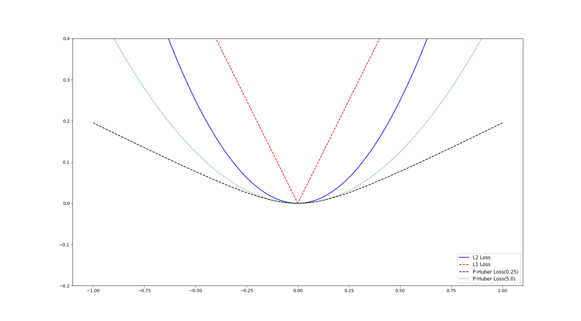
import matplotlib.pyplot as plt import tensorflow as tf   sess = tf.Session() x_vals = tf.linspace(-1., 1., 500) target = tf.constant(0.)   l2_y_vals = tf.square(target - x_vals) l2_y_out = sess.run(l2_y_vals)   l1_y_vals = tf.abs(target - x_vals) l1_y_out = sess.run(l1_y_vals)   delta1 = tf.constant(0.25) phuber1_y_als = tf.multiply(tf.square(delta1), tf.sqrt(1. + tf.square((target - x_vals) / delta1)) - 1.) phuber1_y_out = sess.run(phuber1_y_als)   delta2 = tf.constant(5.) phuber2_y_als = tf.multiply(tf.square(delta2), tf.sqrt(1. + tf.square((target - x_vals) / delta2)) - 1.) phuber2_y_out = sess.run(phuber2_y_als)   # x_array = sess.run(x_vals) # plt.plot(x_array, l2_y_out, 'b-', label='L2 Loss') # plt.plot(x_array, l1_y_out, 'r--', label='L1 Loss') # plt.plot(x_array, phuber1_y_out, 'k--', label='P-Huber Loss(0.25)') # plt.plot(x_array, phuber2_y_out, 'g:', label='P-Huber Loss(5.0)') # plt.ylim(-0.2, 0.4) # plt.legend(loc='lower right', prop={'size': 11}) # plt.show()   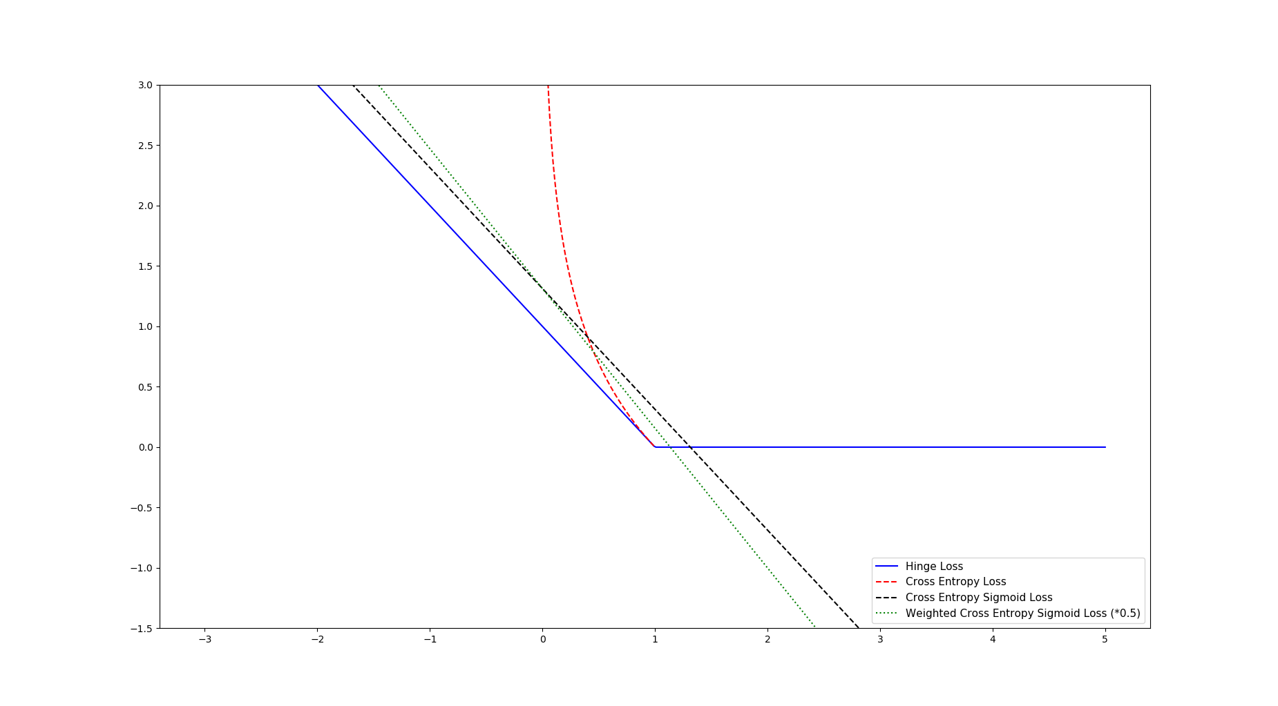x_vals = tf.linspace(-3., 5., 500) target = tf.constant(1.) targets = tf.fill([500, ], 1.)   hinge_y_vals = tf.maximum(0., 1. - tf.multiply(target, x_vals)) hinge_y_out = sess.run(hinge_y_vals)   # [i for i  in xentropy_y_out if not sess.run(tf.is_nan(i))] xentropy_y_vals = -tf.multiply(target, tf.log(x_vals)) - tf.multiply((1. - target), tf.log(1. - x_vals)) xentropy_y_out = sess.run(xentropy_y_vals) not_nan = [i for i in xentropy_y_out if not sess.run(tf.is_nan(i))]   # logits and targets must have the same type and shape. # ValueError: Only call `sigmoid_cross_entropy_with_logits` with named arguments (labels=..., logits=..., ...) xentropy_sigmoid_y_vals = tf.nn.sigmoid_cross_entropy_with_logits(labels=x_vals, logits=targets) xentropy_sigmoid_y_out = sess.run(xentropy_sigmoid_y_vals)   weight = tf.constant(0.5) xentropy_weigthed_y_vals = tf.nn.weighted_cross_entropy_with_logits(x_vals, targets, weight) xentropy_weigthed_y_out = sess.run(xentropy_weigthed_y_vals)   x_array = sess.run(x_vals) plt.plot(x_array, hinge_y_out, 'b-', label='Hinge Loss') plt.plot(x_array, xentropy_y_out, 'r--', label='Cross Entropy Loss') plt.plot(x_array, xentropy_sigmoid_y_out, 'k--', label='Cross Entropy Sigmoid Loss') plt.plot(x_array, xentropy_weigthed_y_out, 'g:', label='Weighted Cross Entropy Sigmoid Loss (*0.5)') plt.ylim(-1.5, 3) plt.legend(loc='lower right', prop={'size': 11}) plt.show()   # unscaled_logits = tf.constant([1., -3., 10.]) # target_dist = tf.constant([0.1, 0.02, 0.88]) # softmax_xentropy = tf.nn.softmax_cross_entropy_with_logits_v2(labels=unscaled_logits, logits=target_dist) # print(sess.run(softmax_xentropy)) # softmax_xentropy_out = sess.run(softmax_xentropy) # # unscaled_logits = tf.constant([1., -3., 10.]) # sparse_target_dist = tf.constant([2]) # sparse_xentropy = tf.nn.sparse_softmax_cross_entropy_with_logits(labels=unscaled_logits, logits=sparse_target_dist) # print(sess.run(sparse_xentropy)) # sparse_xentropy_out = sess.run(sparse_xentropy) dd = 9