
特征向量-Eigenvalues_and_eigenvectors#Graphs 线性变换
总结:
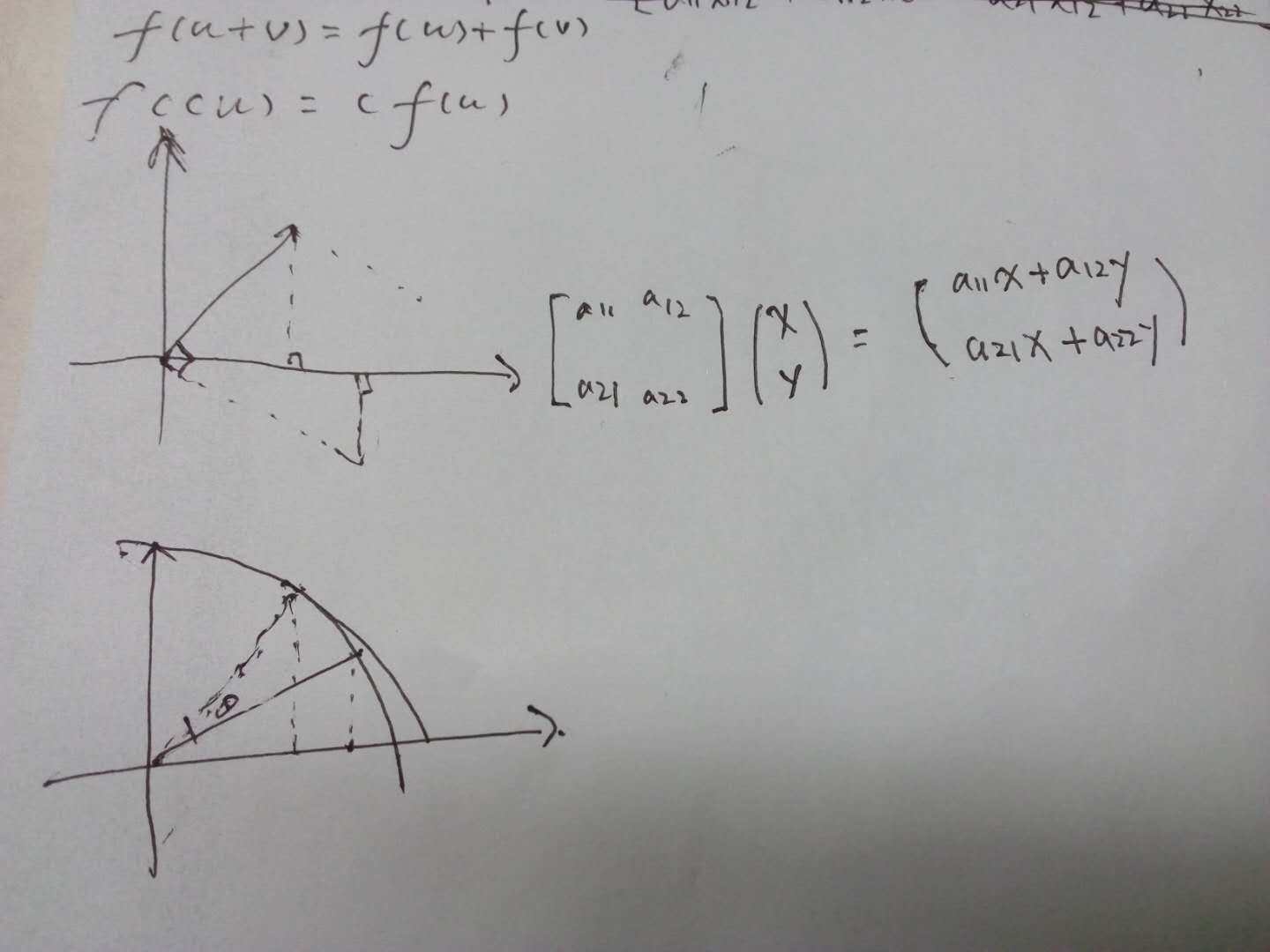
1、线性变换运算封闭,加法和乘法
2、特征向量经过线性变换后方向不变
https://en.wikipedia.org/wiki/Linear_map
Examples of linear transformation matrices
In two-dimensional space R2 linear maps are described by 2 × 2 real matrices. These are some examples:
- rotation
- by 90 degrees counterclockwise:
- by an angle θ counterclockwise:
- by 90 degrees counterclockwise:
- reflection
- about the x axis:
- about the y axis:
- about the x axis:
- scaling by 2 in all directions:
- horizontal shear mapping:
- squeeze mapping:
- projection onto the y axis:


In mathematics, a linear map (also called a linear mapping, linear transformation or, in some contexts, linear function) is a mapping V → W between two modules (including vector spaces) that preserves (in the sense defined below) the operations of addition and scalar multiplication.
An important special case is when V = W, in which case the map is called a linear operator,[1] or an endomorphism of V. Sometimes the term linear function has the same meaning as linear map, while in analytic geometry it does not.
A linear map always maps linear subspaces onto linear subspaces (possibly of a lower dimension);[2] for instance it maps a plane through the origin to a plane, straight line or point. Linear maps can often be represented as matrices, and simple examples include rotation and reflection linear transformations.
In the language of abstract algebra, a linear map is a module homomorphism. In the language of category theory it is a morphism in the category of modules over a given ring.
Definition and first consequences
Let 


 |
additivity / operation of addition |
 |
homogeneity of degree 1 / operation of scalar multiplication |
Thus, a linear map is said to be operation preserving. In other words, it does not matter whether you apply the linear map before or after the operations of addition and scalar multiplication.
This is equivalent to requiring the same for any linear combination of vectors, i.e. that for any vectors 


Denoting the zero elements of the vector spaces 


Occasionally, 


A linear map 
These statements generalize to any left-module 

https://en.wikipedia.org/wiki/Eigenvalues_and_eigenvectors#Graphs
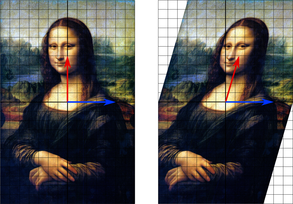
 ,它的特征向量(eigenvector,也译固有向量或本征向量)
 经过这个线性变换
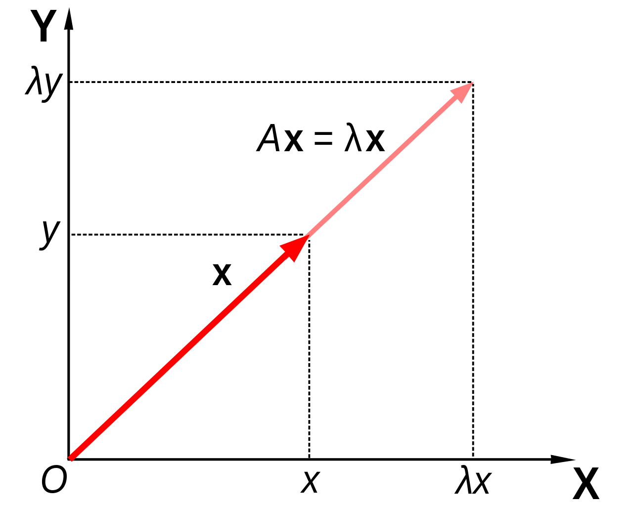
In linear algebra, an eigenvector or characteristic vector of a linear transformation is a non-zero vector that does not change its direction when that linear transformation is applied to it. More formally, if T is a linear transformation from a vector space V over a field F into itself and v is a vector in V that is not the zero vector, then v is an eigenvector of T if T(v) is a scalar multiple of v. This condition can be written as the equation

where λ is a scalar in the field F, known as the eigenvalue, characteristic value, or characteristic root associated with the eigenvector v.
If the vector space V is finite-dimensional, then the linear transformation T can be represented as a square matrix A, and the vector v by a column vector, rendering the above mapping as a matrix multiplication on the left hand side and a scaling of the column vector on the right hand side in the equation

There is a correspondence between n by n square matrices and linear transformations from an n-dimensional vector space to itself. For this reason, it is equivalent to define eigenvalues and eigenvectors using either the language of matrices or the language of linear transformations.[1][2]
Geometrically an eigenvector, corresponding to a real nonzero eigenvalue, points in a direction that is stretched by the transformation and the eigenvalue is the factor by which it is stretched. If the eigenvalue is negative, the direction is reversed.[3]
math.mit.edu/~gs/linearalgebra/ila0601.pdf
A100 was found by using the eigenvalues of A, not by multiplying 100 matrices.
 ,
,
 为
为

 浙公网安备 33010602011771号