2022-2023 春学期 矩阵与数值分析 数值实验大作业
 数值实验大作业
2022-2023 春学期 矩阵与数值分析 数值实验大作业
数值实验大作业题目
《计算机科学计算》第二版 张宏伟等 编著 高等教育出版社
第162页 第四章课后习题第12(1)题、第16题
第216页 第六章课后习题第12题
《数值分析方法与应用》,张宏伟、孟兆良编著;大连理工大学出版社
第214页:
一、基础知识部分
1、5
二、线性方程组求解
2、6
三、非线性方程组求解
1、4
四、插值与逼近
1、5、7
五、数值积分
2
六、微分方程数值解法
1
实验程序环境
# colab
# python 3.10
import math
from math import exp
from math import pow
from math import sqrt
from math import sin
from math import cos
from math import pi
import matplotlib.pyplot as plt
import numpy as np
import sympy
1.1 第四章课后题 12(1)
题目:
用 Newton 法求下列方程的根,要求 \(|x_k-x_{k-1}|<10^{-5}\)
(2) \(x=e^{-x}\),取 \(x_0=0.6\)
程序
def f(x):
  return exp(-x)-x
def df(x):
  return -exp(-x)-1
def Newton(f,df):
  x0 = 0.6
  x1 = 0
  t = abs(x1 - x0)
  while t >= 1e-5:
    x1 = x0-f(x0)/df(x0)
    t = abs(x1-x0)
    print(*[x1,x0,t])
    x0 = x1

  return x0
Newton(f,df)
输出
0.5669499100387272 0.6 0.03305008996127279
0.5671432836426546 0.5669499100387272 0.00019337360392746028
0.5671432904097838 0.5671432836426546 6.767129190343724e-09
0.5671432904097838
1.2 第四章课后题 16
题目:
Heonardo 于 1225 年研究了方程
并得出一个根 \(\alpha=1.36880817\),但当时无人知道他用了什么方法,这个结果在当时是个非常著名的结果,请你构造一种简单迭代来验证此结果.
程序
def f(x):
  return pow(x,3)+2*pow(x,2)+10*x-20
def df(x):
  return 3*pow(x,2)+4*x+10
def Newton(f,df):
  x0 = 1
  x1 = 0
  t = abs(x1 - x0)
  while t >= 1e-10:
    x1 = x0-f(x0)/df(x0)
    t = abs(x1-x0)
    print(*[x1,x0,t])
    x0 = x1

  return x0
Newton(f,df)
输出
1.4117647058823528 1 0.4117647058823528
1.3693364705882352 1.4117647058823528 0.042428235294117655
1.3688081886175318 1.3693364705882352 0.0005282819707033148
1.3688081078213745 1.3688081886175318 8.0796157320151e-08
1.3688081078213727 1.3688081078213745 1.7763568394002505e-15
1.3688081078213727
1.3 第六章课后题 12
题目:
(数值实验题)人造卫星的轨道可视为平面上的椭圆,地心位于椭圆的一个焦点处。已知一颗人造卫星近地点距地球表面 439km,远地点距地球表面 2384km,地球半径为 6371km,求该卫星的轨道长度
程序
er = 6371
lr = 2384
sr = 439

a = (2*er+lr+sr)/2.
c = a - sr - er/2.
b = sqrt(pow(a,2)-pow(c,2))
e = c/a

# xmpy = sympy.Symbol('x')
# print("true value\t{:s}".format(str(sympy.integrate(4*a*sympy.sqrt((1-sympy.Pow(e,2)*sympy.Pow(xmpy,2))/(1-sympy.Pow(xmpy,2))),(xmpy,0,1.)))))
# (sympy.integrate(4*a*sympy.sqrt((1-sympy.Pow(e,2)*sympy.Pow(xmpy,2))/
#  (1-sympy.Pow(xmpy,2))),(xmpy,0,1.)))

def f(x):
  return 4.*a*sqrt((1-pow(e,2)*pow(x,2))/(1-pow(x,2)))
def GaussChebyshev(f):
  return pi/2.*(f(-sqrt(2)/2.)+f(sqrt(2)/2.))
GaussChebyshev(f)
输出
128057.20405940955
2.1 基础知识部分 1
题目:
设 \(S_N=\sum\limits^N_{j=2}\frac{1}{j^2-1}\),其精确值为 \(\frac{1}{2}(\frac{3}{2}-\frac{1}{N}-\frac{1}{N+1})\).
(1)编制按从大到小的顺序 \(S_N=\frac{1}{2^2-1}+\frac{1}{3^2-1}+\cdots+\frac{1}{N^2-1}\),计算 \(S_N\) 的通用程序.
(2)编制按从小到大的顺序 \(S_N=\frac{1}{N^2-1}+\frac{1}{(N-1)^2-1}+\cdots+\frac{1}{2^2-1}\),计算 \(S_N\) 的通用程序.
(3)按两种顺序分别计算,并指出有效位数(编制程序时用单精度).
(4)通过本上机题,你明白了什么.
程序
def sn1(N):
  ans=0
  for i in range(2,N+1):
    ans += 1./(pow(i,2)-1)
  return ans
sn1(2)
输出
0.3333333333333333
程序
def sn2(N):
  ans=0
  for i in range(N,2-1,-1):
    ans += 1./(pow(i,2)-1)
  return ans
sn1(2)
输出
0.3333333333333333
程序
print("从小到大计算 SN,N 从 10 到 10^6 的结果分别为:")
for i in range(1,7):
  print("N=10^"+str(i)+", SN="+str(sn1(int(pow(10.,i)))))
输出
从小到大计算 SN,N 从 10 到 10^6 的结果分别为:
N=10^1, SN=0.6545454545454544
N=10^2, SN=0.7400495049504949
N=10^3, SN=0.7490004995005
N=10^4, SN=0.7499000049995057
N=10^5, SN=0.7499900000500057
N=10^6, SN=0.7499990000005217
程序
print("从大到小计算 SN,N 从 10 到 10^6 的结果分别为:")
for i in range(1,7):
  print("N=10^"+str(i)+", SN="+str(sn2(int(pow(10.,i)))))
输出
从大到小计算 SN,N 从 10 到 10^6 的结果分别为:
N=10^1, SN=0.6545454545454545
N=10^2, SN=0.7400495049504949
N=10^3, SN=0.7490004995004995
N=10^4, SN=0.7499000049995
N=10^5, SN=0.7499900000499995
N=10^6, SN=0.7499990000004999
程序
def sn(N):
  return 1./2.*(3./2.-1./N-1./(N+1))
print("计算 SN 精确值,N 从 10 到 10^6 的结果分别为:")
for i in range(1,7):
  print("N=10^"+str(i)+", SN="+str(sn(int(pow(10.,i)))))
输出
计算 SN 精确值,N 从 10 到 10^6 的结果分别为:
N=10^1, SN=0.6545454545454545
N=10^2, SN=0.740049504950495
N=10^3, SN=0.7490004995004995
N=10^4, SN=0.7499000049995
N=10^5, SN=0.7499900000499995
N=10^6, SN=0.7499990000005
2.2 基础知识部分 5
题目:
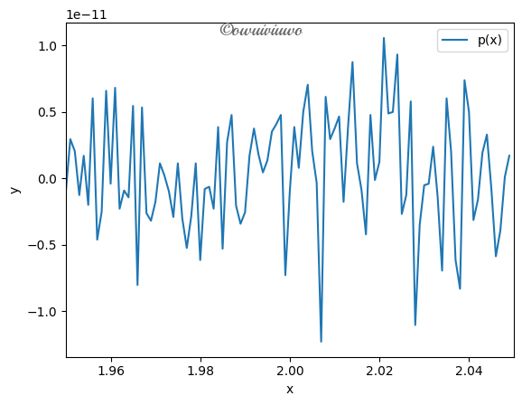
首先编制一个利用秦九韶算法计算一个多项式在给定点的函数值的通用程序,程序包括输入多项式的系数以及给定点,输出函数值,利用编制的程序计算
程序
def qinjiushao(factors, xs):
  # factors 为系数列表,从高次王低次排列
  # xs 为给定点列表
  ans = np.array([])
  for x in xs:
    t = factors[0]
    for f in factors[1:]:
      t = t * x + f
    # ans.append(t)
    ans=np.append(ans,[t])
  return ans
xs = np.arange(1.95,2.05,0.001)
factors = np.array([1,-18,144,-672,2016,-4032,5376,-4608,2304,-512])
y = qinjiushao(factors,xs)
plt.plot(xs, y, label="p(x)")
plt.xlabel("x")
plt.ylabel("y")
plt.xlim(1.95, 2.05)
plt.legend()
plt.show()
print(y)
输出
[-9.66338121e-13  2.95585778e-12  2.04636308e-12 -1.25055521e-12
1.70530257e-12 -1.98951966e-12  6.02540240e-12 -4.60431693e-12
-2.50111043e-12  6.59383659e-12 -3.97903932e-13  6.82121026e-12
-2.27373675e-12 -9.09494702e-13 -1.42108547e-12  5.45696821e-12
-8.01492206e-12  5.34328137e-12 -2.61479727e-12 -3.18323146e-12
-1.76214598e-12  1.13686838e-12  2.27373675e-13 -9.66338121e-13
-2.89901436e-12  1.13686838e-12 -3.01270120e-12 -5.22959454e-12
-2.84217094e-12  1.13686838e-12 -6.13908924e-12 -7.95807864e-13
-6.25277607e-13 -2.27373675e-12  3.86535248e-12 -5.28643795e-12
2.72848411e-12  4.77484718e-12 -2.04636308e-12 -3.41060513e-12
-2.55795385e-12  1.70530257e-12  3.75166564e-12  1.81898940e-12
4.54747351e-13  1.36424205e-12  3.52429197e-12  4.09272616e-12
4.77484718e-12 -7.27595761e-12 -9.66338121e-13  3.86535248e-12
7.95807864e-13  5.00222086e-12  7.04858394e-12  2.04636308e-12
-3.41060513e-13 -1.22781785e-11  6.13908924e-12  2.95585778e-12
3.75166564e-12  4.66116035e-12 -1.76214598e-12  3.86535248e-12
8.75388650e-12  1.13686838e-12 -8.52651283e-13 -4.20641300e-12
4.77484718e-12 -1.13686838e-13  1.25055521e-12  1.05728759e-11
4.88853402e-12  5.00222086e-12  9.32232069e-12 -2.67164069e-12
-1.25055521e-12  5.79802872e-12 -1.10276233e-11 -3.46744855e-12
-5.11590770e-13 -3.97903932e-13  2.38742359e-12 -1.36424205e-12
-6.93489710e-12  6.02540240e-12  2.04636308e-12 -6.13908924e-12
-8.29913915e-12  7.38964445e-12  5.00222086e-12 -3.12638804e-12
-1.59161573e-12  1.93267624e-12  3.29691829e-12 -7.95807864e-13
-5.85487214e-12 -3.92219590e-12  1.13686838e-13  1.70530257e-12]
2.3 线性方程组求解 2
题目:
编制程序求解矩阵 A 的 Choleskey 分解,并用程序求解方程组 Ax=b,其中
注:书上原矩阵为 \(A=\begin{pmatrix}2&1&-5&1\\1&-5&2&7\\0&2&1&-1\\1&7&-1&-4\end{pmatrix}\),不符合课程中有关对称正定矩阵的 Choleskey 分解的要求,因此依据某版本勘误,修改为本题中矩阵。
程序
A = np.array([[7,1,-5,1],[1,9,2,7],[-5,2,7,-1],[1,7,-1,9]])
b = np.array([[13,-9,6,0]]).T
def Choleskey(A):
  ans = np.zeros(A.shape)
  for j in range(A.shape[0]):
    for i in range(j, A.shape[0]):
      t = 0
      for k in range(0,j):
        t += pow(ans[j][k],2)
      ans[j][j] = sqrt(A[j][j]-t)
      t = 0
      for k in range(0,j):
        t += ans[i][k]*ans[j][k]
      ans[i][j] = (A[i][j]-t)/ans[j][j]
  return ans

# L = Choleskey(A_)
L = Choleskey(A)
print("L=")
print(L)

def Lyb(L,b):
  y = np.zeros(b.shape)
  for i in range(b.shape[0]):
    t=0
    for k in range(i):
      t += L[i][k] * y[k][0]
    y[i][0] = (b[i][0]-t)/L[i][i]
  return y
y = Lyb(L,b)
print('y=')
print(y)

def LTxy(L,y):
  x = np.zeros(y.shape)
  for i in range(L.shape[0]-1,0-1,-1):
    t = 0
    for k in range(i,L.shape[0]):
      t += L[k][i] * x[k][0]
    x[i][0] = (y[i][0]-t)/L[i][i]
  return x
x = LTxy(L,y)
print('x=')
print(x)
输出
L=
[[ 2.64575131  0.          0.          0.        ]
[ 0.37796447  2.97609524  0.          0.        ]
[-1.88982237  0.91202919  1.61145096  0.        ]
[ 0.37796447  2.30407373 -1.4813338   1.16363107]]
y=
[[ 4.91353815]
[-3.64811674]
[11.55040004]
[20.33151718]]
x=
[[ 19.07798165]
[-21.87155963]
[ 23.2293578 ]
[ 17.47247706]]
2.4 线性方程组求解 6
题目:
令 \(H\) 表示 \(n\times n\) 的 Hilbert 矩阵,其中 \((i,j)\) 元素是 \(1/(i+j-1)\),b 是元素全为 1 的向量,用 Gauss 消去法求解 Hx=b,其中取
(1) n=2;
(2) n=5;
(3) n=10;
程序
def Hilbert(n):
  ans = np.zeros((n,n))
  for i in range(n):
    for j in range(n):
      ans[i][j] = 1./(i+1+j+1-1)
  return ans

def Gauss(A,b):
  ans = np.zeros(b.shape)
  n = A.shape[0]
  Ab = np.hstack((A,b))

  for j in range(0,n-1):
    for i in range(j+1,n):
      Ab[i] = Ab[i] - Ab[j] * Ab[i][j]/Ab[j][j]
  # print(Ab)
  for i in range(n-1,-1,-1):
    t = 0
    for j in range(i+1,n):
      t += ans[j][0] * Ab[i][j]

    ans[i][0] =  (Ab[i][n] - t)/Ab[i][i]
    # print((i,b[i][0]))
  return ans

for i in [2,5,10]:
  x = Gauss(Hilbert(i), np.ones((i,1)))
  print("Hx=b, H=Hilbert({:d}),b 是元素全为 1 的向量".format(i))
  print(x)
输出
Hx=b, H=Hilbert(2),b 是元素全为 1 的向量
[[-2.]
[ 6.]]
Hx=b, H=Hilbert(5),b 是元素全为 1 的向量
[[    5.]
[ -120.]
[  630.]
[-1120.]
[  630.]]
Hx=b, H=Hilbert(10),b 是元素全为 1 的向量
[[-9.99726592e+00]
[ 9.89763037e+02]
[-2.37549411e+04]
[ 2.40193928e+05]
[-1.26103993e+06]
[ 3.78317436e+06]
[-6.72572540e+06]
[ 7.00031810e+06]
[-3.93771469e+06]
[ 9.23668814e+05]]
2.5 非线性方程组求解 1
题目:
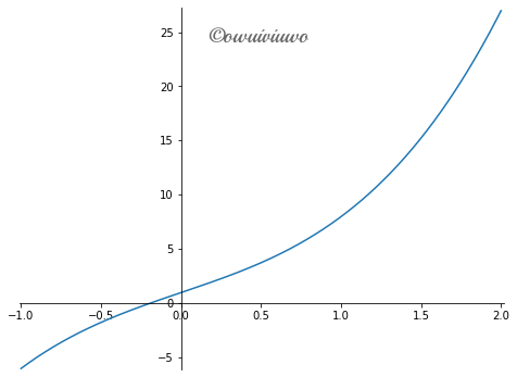
分别应用 Newton 迭代法和割线法计算
(1)非线性方程 \(2x^3+5x+1=0\) 在 \([1,2]\) 上的一个根
(2)\(e^x\sin x=0\) 在 \([-4,-3]\) 上的一个根
程序
def f1(x):
  return 2*pow(x,3)+5*x+1
def df1(x):
  return 6*x + 5
def f2(x):
  return exp(x)*sin(x)
def df2(x):
  return exp(x)*sin(x)+exp(x)*cos(x)
def Newton(f,df,y,lb,rb):
  x = (lb+rb)/2.
  while abs(f(x)-y)>1e-10:
    x = x-f(x)/df(x)
  return x
def cutlines(f,y,lb,rb):
  x0=np.random.uniform(lb,rb)
  x1=np.random.uniform(x0,rb)
  x = x1
  while abs(f(x)-y)>1e-10:
    x = x1 - (x1-x0)*f(x1)/(f(x1)-f(x0))
    x0 = x1
    x1 = x
  return x
#(1)
print('(1)')
print('Newton 法: '+str(Newton(f1,df1,0.,1.,2.)))
print('割线法: '+str(cutlines(f1,0.,1.,2.)))
#(2)
print('(2)')
print('Newton 法: '+str(Newton(f2,df2,0.,-4.,-3.)))
print('割线法: '+str(cutlines(f2,0.,-4.,-3.)))

np.random.uniform(1,2)
xt = np.arange(-1,2,0.001)
yt = np.array([f1(i) for i in xt])
def pltshow(X,Y):
  fig = plt.figure(figsize=(8,6), dpi=72,facecolor="white")
  axes = plt.subplot(111)
  axes.plot(X,Y)#, color = 'blue', linewidth=2, linestyle="-")
  axes.set_xlim(1.01*X.min(),1.01*X.max())
  axes.set_ylim(1.01*Y.min(),1.01*Y.max())

  axes.spines['right'].set_color('none')
  axes.spines['top'].set_color('none')
  axes.xaxis.set_ticks_position('bottom')
  axes.spines['bottom'].set_position(('data',0))
  axes.yaxis.set_ticks_position('left')
  axes.spines['left'].set_position(('data',0))
  plt.show()
pltshow(xt,yt)
输出
(1)
Newton 法: -0.1969444376699362
割线法: -0.19694443765320088
(2)
Newton 法: -3.141592653579501
割线法: -3.1415926535895866
2.6 非线性方程组 4
题目:
用 Newton 迭代法求解方程 \(x^3+x^2+x-3=0\) 的根,初值选择 \(x_0=-0.7\),迭代 7 步并与真值 相比较,并列出数据表
| \(i\) | \(x_i\) | \(e_i=|x_i-x^*|\) | \(\frac{e_i}{e_2^{i-1}}\) |
| :--: | :---: | :-------------: | :---------------------: |
| 0 | | | |
| 1 | | | |
| 2 | | | |
程序
def Newton7(f,df,y,xtrue=1):
  x = -0.7
  c = 0
  e = abs(x - xtrue)

  print(*[c,x,e,e/pow(e,2)])
  while abs(f(x)-y)>1e-10 and c < 11:

    x = x-f(x)/df(x)
    c += 1
    e = abs(x-xtrue)
    print(*[c,x,e,e/pow(e,2)])

  return x
def f(x):
  return pow(x,3)+pow(x,2)+x-3
def df(x):
  return 3*pow(x,2)+2*x+1
Newton7(f,df,0)
输出
0 -0.7 1.7 0.5882352941176471
1 2.6205607476635517 1.6205607476635517 0.6170703575547865
2 1.7084401902625614 0.7084401902625614 1.4115517636420105
3 1.2063786980181086 0.2063786980181086 4.845461327177554
4 1.024161664125103 0.02416166412510301 41.387877706694866
5 1.0003814911210203 0.00038149112102026095 2621.2929866509007
6 1.0000000969928142 9.699281422470563e-08 10310042.120061344
7 1.0000000000000062 6.217248937900877e-15 160842843834660.56
1.0000000000000062
2.7 插值与逼近 1
题目:
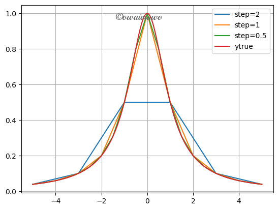
已知函数 \(f(x)=\frac{1}{1+x^2}\),在 \([-5,5]\) 上分别取 \(2,1,\frac{1}{2}\) 为单位长度的等距节点作为插值节点,用 Lagrange 方法插值,并把原函数图与插值函数图比较,观察插值效果
程序
def f(x):
  return 1./(1+np.power(x,2))

x = np.array(
    [np.arange(-5,5.1,2.),
    np.arange(-5,5.1,1.),
    np.arange(-5,5.1,0.5)]
)

y = f(x)

def LagrangeInterpolation(x,y):
  def ans(x_):
    res = 0
    n = y.shape[0];
    L = np.ones(n)
    for i in range(n):
      for j in range(n):
        if j != i:
          L[i] *= (x_ - x[j])
          L[i] /= (x[i] - x[j])
      L[i] *= y[i]
    return L.sum()
  return ans

for i in range(3):
  L = LagrangeInterpolation(x[i],y[i])
labels=[
    'step=2','step=1','step=0.5'
]
for i,j,k in zip(x,y,labels):
  plt.plot(i,j,label=k)
xtrue = np.arange(-5,5.0001,0.01)
ytrue = f(xtrue)
plt.plot(xtrue,ytrue,label='ytrue')
plt.legend()
plt.grid()
plt.show()
输出
    <ipython-input-18-04d7d62ca026>:4: VisibleDeprecationWarning: Creating an ndarray from ragged nested sequences (which is a list-or-tuple of lists-or-tuples-or ndarrays with different lengths or shapes) is deprecated. If you meant to do this, you must specify 'dtype=object' when creating the ndarray.
      x = np.array(
2.8 插值与逼近 5
题目:
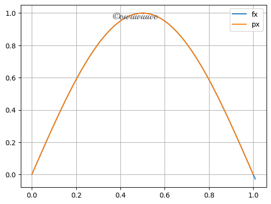
考虑函数 \(f(x)=\sin\pi x,x\in[0,1]\),用等距节点作\(f(x)\)的Newton插值,画出插值多项式以及\(f(x)\)的图像,观察收敛性
程序
def f(x):
  return np.sin(pi*x)
def NewtonInterpolation(x,y,h):

  res = 0.
  n = x.shape[0]
  # DD = np.zeros((n+1,n))
  # DD[0] = x
  # DD[1] = y
  DD = np.zeros((n,n))
  DD[0] = y
  DD = DD.T
  # print(DD)
  # for i in range(2,n+1):
  #   for j in range(i-1,n):
  #     DD[j][i] = (DD[j][i-1]-DD[j-1][i-1])/((i-1)*h)
  # print(DD)
  for i in range(1,n):
    for j in range(i,n):
      DD[j][i] = (DD[j][i-1]-DD[j-1][i-1])/((i)*h)
  # print(DD)
  def ans(x_):
    res=0
    res += DD[0][0]
    for i in range(1,n):
      t = 1
      for j in range(i):
        t *= (x_-x[j])
      res += DD[i][i] * t
    return res
  return ans
h=0.001
x = np.arange(0,1.01,h)
y = f(x)
plt.plot(x,y,label='fx')

h=0.02
x = np.arange(0,1.01,h)
y = f(x)
p = NewtonInterpolation(x,y,h)
py = p(x)

plt.plot(x,py,label='px')
plt.legend()
plt.grid()
plt.show()
输出
2.9 插值与逼近 7
题目:
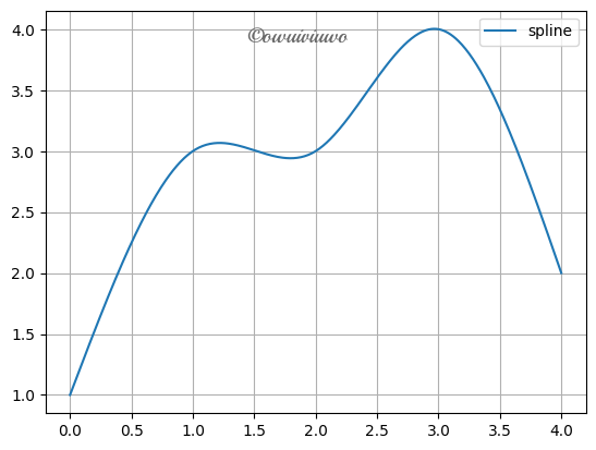
编程计算三次样条 S,满足 \(S(0)=1,S(1)=3,S(2)=3,S(3)=4,S(4)=2\),其中边界条件\(S''(0)=S''(4)=0\)
程序
def NaturalCubicSpline(x,y):
  # p149-p150; algorithm 3.4; Numerical Analysis 9th Autor: Richard L.Burden and J.Douglas Faires
  n = x.shape[0] - 1
  h = np.zeros((n,))
  abcd = np.zeros((n,n+1))
  abcd = abcd.T
  a,b,c,d = y,np.zeros((n+1,)),np.zeros((n+1,)),np.zeros((n+1,))
  # step 1
  for i in range(0,n):
    h[i] = x[i+1]-x[i]
  # step 2
  alpha = np.zeros((n,))
  for i in range(1,n):
    alpha[i]=3./h[i]*(a[i+1]-a[i])-3./h[i-1]*(a[i]-a[i-1])
  # step 3
  L,u,z = np.zeros((n+1,)),np.zeros((n+1,)),np.zeros((n+1,))
  L[0] = 1
  u[0] = 0
  z[0] = 0
  # step 4
  for i in range(1,n):
    L[i]=2*(x[i+1]-x[i-1])-h[i-1]*u[i-1]
    u[i]=h[i]/L[i]
    z[i]=(alpha[i]-h[i-1]*z[i-1])/L[i]
  # step 5
  L[n]=1
  z[n]=0
  c[n]=0
  # step 6
  for j in range(n-1,-1,-1):
    c[j]=z[j]-u[j]*c[j+1]
    b[j]=(a[j+1]-a[j])/h[j]-h[j]*(c[j+1]+2*c[j])/3.
    d[j]=(c[j+1]-c[j])/(3.*h[j])
  # print(a)
  # print(b)
  # print(c)
  # print(d)
  abcd[0]=a[:-1]
  abcd[1]=b[:-1]
  abcd[2]=c[:-1]
  abcd[3]=d[:-1]
  abcd = abcd.T
  print(abcd)
  def spline(x_):
    res = 0
    t = x[0]
    for i in range(n):
      # print((x_,x[i],x[i+1]))
      if x_ >= x[i] and x_ <= x[i+1]:
        t = i
        break
    for i in range(n+1):
      res += abcd[t][i] * pow(x_-x[t],i)
    return res
  return spline
x = np.array([0.,1.,2.,3.,4.])
y = np.array([1.,3.,3.,4.,2.])
spl = NaturalCubicSpline(x,y)
x_ = np.arange(0,4.01,0.01)
y_ = [spl(i) for i in x_]
plt.plot(x_,y_,label='spline')
plt.grid()
plt.legend()
plt.show()
输出
[[ 1.          2.66071429  0.         -0.66071429  0.        ]
[ 3.          0.67857143 -1.98214286  1.30357143  0.        ]
[ 3.          0.625       1.92857143 -1.55357143  0.        ]
[ 4.         -0.17857143 -2.73214286  0.91071429  0.        ]]
2.10 数值积分 2
题目:
用两点,三点和五点的Gauss型积分公式分别计算定积分,并与真值作比较
本题使用 Gauss-Legendre 公式,通过查表可知对应的系数以及 Gauss 点如下表所示:
| \(n\) | Roots \(r_{n,i}\) | Coefficients \(c_{n,j}\) |
|---|---|---|
| 2 | 0.5773502692 | 1.0000000000 |
| −0.5773502692 | 1.0000000000 | |
| 3 | 0.7745966692 | 0.5555555556 |
| 0.0000000000 | 0.8888888889 | |
| −0.7745966692 | 0.5555555556 | |
| 4 | 0.8611363116 | 0.3478548451 |
| 0.3399810436 | 0.6521451549 | |
| −0.3399810436 | 0.6521451549 | |
| −0.8611363116 | 0.3478548451 | |
| 5 | 0.9061798459 | 0.2369268850 |
| 0.5384693101 | 0.4786286705 | |
| 0.0000000000 | 0.5688888889 | |
| −0.5384693101 | 0.4786286705 | |
| −0.9061798459 | 0.2369268850 |
程序
xmpy = sympy.Symbol('x')
print("true value\t{:s}".format(str(sympy.integrate(sympy.cos(xmpy)*xmpy*xmpy,(xmpy,0,pi/2.)))))

def f(x):
  return pow(x,2)*cos(x)
def GaussLegendreIntergrate(f,x,coefficients):
  res = 0
  for i,j in zip(x,coefficients):
    res += f(i)*j
  return res
# n=2
x=[0.5773502692,-0.5773502692]
coefficients=[1.0000000000,1.0000000000]
print("n=2,\t\t{:s}".format(str(GaussLegendreIntergrate(f,x,coefficients))))
# n=3
x=[0.7745966692,0.0000000000,-0.7745966692]
coefficients=[0.5555555556,0.8888888889,0.5555555556]
print("n=3,\t\t{:s}".format(str(GaussLegendreIntergrate(f,x,coefficients))))
# n=5
x=[0.9061798459, 0.5384693101, 0.0000000000, -0.5384693101, -0.9061798459]
coefficients=[ 0.236926885, 0.4786286705, 0.5688888889, 0.4786286705, 0.2369268850]
print("n=5,\t\t{:s}".format(str(GaussLegendreIntergrate(f,x,coefficients))))
输出
true value	0.467401100272340
n=2,		0.5586078851462954
n=3,		0.476468795309243
n=5,		0.4782671832477956
2.11 微分方程数值解法 1
题目:
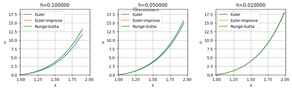
已知常微分方程
分别用Euler法,改进的Euler法,Runge-Kutta法求解该方程,步长选为0.1,0.05,0.01,画图观察求解效果
程序
hs=[0.1,0.05,0.01]
def f(u,x):
  return 2.*u/x+pow(x,2)*exp(x)
def Euler(u,h,x,f):
  return u+h*f(u,x)
def EulerImprove(u,h,x,f,*args):
  u_=u+h*f(u,x)
  return u+h/2.*(f(u,x)+f(u,x+h))
def RungeKutta(u,h,x,f):
  # 4 阶
  # p288-p289; algorithm 5.2; Numerical Analysis 9th Autor: Richard L.Burden and J.Douglas Faires
  # 此处课件与上述参考书目不同,课件中 k2,k3,k4 的 u 的迭代过程多乘了一个 h
  # 可与下一单元格中对应位置作对比
  k1 = h*f(u,x)
  k2 = h*f(u+h*k1/2.,x+h/2.)
  k3 = h*f(u+h*k2/2.,x+h/2.)
  k4 = h*f(u+h*k3,x+h)
  return u + (k1+2*k2+2*k3+k4)/6.


functions=[Euler,EulerImprove,RungeKutta]
labels = ['Euler','Euler-improve','Runge-kutta']
fig = plt.figure(figsize=(12,3))
fig.subplots_adjust(hspace=0.4, wspace=0.4)
for h in hs:
  # axes = plt.subplot()
  # axes.set_xlim(0.99,2.01)
  # axes
  subplot = plt.subplot(1,3,hs.index(h)+1)
  subplot.set_xlim(0.99,2.01)
  subplot.set_ylim(-0.01,19.)
  for fun,label in zip(functions,labels):
    x = 1
    u1 = 0
    us = []
    xs = []
    while x < 2:
      us.append(u1)
      xs.append(x)
      u2 = fun(u1,h,x,f)
      x += h
      u1 = u2
    # plt.subplot(1,3,hs.index(h)+1)
    plt.plot(xs,us,label = label)

  plt.title("h={:f}".format(h))
  plt.xlabel("x")
  plt.ylabel("u")
  plt.legend()
  plt.grid()
plt.show()
输出
程序
x=np.arange(0,2,0.2)
x = 0.
u1 = 0.5
h = 0.2
def RungeKutta(u,h,x,f):
  # 4 阶
  # p288-p289; algorithm 5.2; Numerical Analysis 9th Autor: Richard L.Burden and J.Douglas Faires
  # 此处课件与上述参考书目不同,参考书目中 k2,k3,k4 的 u 的迭代过程少乘了一个 h
  # 可与上一单元格中对应位置作对比
  k1 = h*f(u,x)
  k2 = h*f(u+k1/2.,x+h/2.)
  k3 = h*f(u+k2/2.,x+h/2.)
  k4 = h*f(u+k3,x+h)
  print((k1,k2,k3,k4))
  return u + (k1+2*k2+2*k3+k4)/6.
def f(u,x):
  return u-pow(x,2)+1
while x < 2:
  print(u1)
  u2 = RungeKutta(u1,h,x,f)
  x += h
  u1 = u2
输出
0.5
(0.30000000000000004, 0.32800000000000007, 0.3308, 0.35816000000000003)
0.8292933333333334
(0.3578586666666667, 0.38364453333333337, 0.38622312000000003, 0.41110329066666673)
1.2140762106666667
(0.4108152421333333, 0.4338967663466667, 0.43620491876800005, 0.4580562258869334)
1.6489220170416001
(0.45778440340832005, 0.477562843749152, 0.4795406877832353, 0.49769254096496707)
2.1272026849479437
(0.49744053698958873, 0.5131845906885476, 0.5147589960584436, 0.5283923362012776)
2.6408226927287517
(0.5281645385457504, 0.5389809924003254, 0.5400626377857828, 0.548177066102907)
3.1798941702322305
(0.5479788340464461, 0.5527767174510906, 0.5532565057915552, 0.5546301352047571)
3.7323400728549796
(0.5544680145709959, 0.5519148160280957, 0.5516594961738054, 0.544799913805757)
4.283409498318406
(0.5446818996636813, 0.5331500896300494, 0.5319969086266862, 0.5150812813890185)
4.815085694579435
(0.5150171389158871, 0.4925188528074757, 0.4902690241966345, 0.46107094375521407)
5.305363000692655
(0.46107260013853113, 0.42517986015238435, 0.42159058615376976, 0.3773907173692852)

