HITNet_Hierarchical_Iterative_Tile_Refinement_Network_for_Real-time_Stereo
 本文提出了HITNet,一种用于实时立体匹配的新型神经网络架构。与许多近期在全代价体上运行并依赖${3D}$卷积的神经网络方法不同,我们的方法并不显式构建代价体,而是依靠快速多分辨率初始化步骤、可微的${2D}$几何传播和变形机制来推断视差假设。为了达到较高的精度,我们的网络不仅从几何角度推理视差,还推断倾斜平面假设,从而能够更准确地执行几何变形和上采样操作。我们的架构本质上是多分辨率的,允许信息在不同层次之间传播。多项实验证明,与最先进的方法相比,所提出的方法在所需计算量大幅减少的情况下仍具有有效性。
| 英文题目 | HITNet: Hierarchical Iterative Tile Refinement Network for Real-time Stereo Matching |
|---|---|
| 中文名称 | HITNet:用于实时立体匹配的分层迭代图块细化网络 |
| 发表时间 | 2020年7月23日 |
| 平台 | CVPR 2021 |
| 作者 | Vladimir Tankovich, Christian Häne, Yinda Zhang, Adarsh Kowdle, Sean Fanello, Sofien Bouaziz |
| 邮箱 | {vtankovich, chaene, yindaz, adarshkowdle, seanfa, sofien}@google.com |
| 来源 | |
| 关键词 | Real-time Stereo Matching |
| paper && code && video | paper code video |
Abstract
摘要
This paper presents HITNet, a novel neural network architecture for real-time stereo matching. Contrary to many recent neural network approaches that operate on a full cost volume and rely on \({3D}\) convolutions, our approach does not explicitly build a volume and instead relies on a fast multi-resolution initialization step, differentiable \({2D}\) geometric propagation and warping mechanisms to infer disparity hypotheses. To achieve a high level of accuracy, our network not only geometrically reasons about disparities but also infers slanted plane hypotheses allowing to more accurately perform geometric warping and upsampling operations. Our architecture is inherently multi-resolution allowing the propagation of information across different levels. Multiple experiments prove the effectiveness of the proposed approach at a fraction of the computation required by state-of-the-art methods. At the time of writing, HITNet ranks \({1}^{\text{st }}\) - \({3}^{rd}\) on all the metrics published on the ETH3D website for two view stereo, ranks \({1}^{\text{st }}\) on most of the metrics amongst all the end-to-end learning approaches on Middlebury-v3, ranks \({1}^{\text{st }}\) on the popular KITTI 2012 and 2015 benchmarks among the published methods faster than \({100}\mathrm{{ms}}\) .
- 本文提出了HITNet,一种用于实时立体匹配的新型神经网络架构。
- 与许多近期在 a full cost volume 上运行并依赖\({3D}\)卷积的神经网络方法不同,我们的方法并不显式构建 a volume,而是依靠快速多分辨率初始化步骤、可微的\({2D}\)几何传播和变形机制来推断视差假设。
- 为了达到较高的精度,我们的网络不仅从几何角度推理视差,还推断倾斜平面假设,从而能够更准确地执行几何变形和上采样操作。
- 我们的架构本质上是多分辨率的,允许信息在不同层次之间传播。
- 多项实验证明,与最先进的方法相比,所提出的方法在所需计算量大幅减少的情况下仍具有有效性。
- 在撰写本文时,HITNet在ETH3D网站发布的双目立体视觉的所有指标中排名\({1}^{\text{st }}\) - \({3}^{rd}\),在Middlebury - v3的所有端到端学习方法的大多数指标中排名\({1}^{\text{st }}\),在比\({100}\mathrm{{ms}}\)更快的已发布方法中,在流行的KITTI 2012和2015基准测试中排名\({1}^{\text{st }}\)。
1. Introduction
1. 引言
Recent research on depth from stereo matching has largely focused on developing accurate but computationally expensive deep learning approaches. Large convolutional neural networks (CNNs) can often use up to a second or even more to process an image pair and infer a disparity map. For active agents such as mobile robots or self driving cars such a high latency is undesirable and methods which are able to process an image pair in a matter of milliseconds are required instead. Despite this, only 4 out of the top 100 methods on the KITTI 2012 leaderboard are published approaches that take less than \({100}{\mathrm{{ms}}}^{1}\) .
近期关于立体匹配深度估计的研究主要集中在开发准确但计算成本高的深度学习方法上。大型卷积神经网络(CNN)通常需要一秒甚至更长时间来处理一对图像并推断视差图。对于移动机器人或自动驾驶汽车等主动智能体来说,如此高的延迟是不可取的,相反,需要能够在几毫秒内处理一对图像的方法。尽管如此,在KITTI 2012排行榜的前100种方法中,只有4种已发布的方法处理时间少于\({100}{\mathrm{{ms}}}^{1}\)。
\({}^{1}\) Additional approaches faster than \({100}\mathrm{\;{ms}}\) are on the leaderboard but the algorithms are unpublished and hence it is unknown how the results were achieved.
\({}^{1}\) 比\({100}\mathrm{\;{ms}}\)更快的其他方法排在排行榜上,但这些算法未发表,因此不清楚这些结果是如何获得的。
A common pattern in end-to-end learning based approaches to computational stereo is utilizing a CNN which is largely unaware of the geometric properties of the stereo matching problem. In fact, initial end-to-end networks were based on a generic U-Net architecture [38]. Subsequent works have pointed out that incorporating explicit matching cost volumes encoding the cost of assigning a disparity to a pixel, in conjunction with \(3\mathrm{D}\) convolutions provides a notable improvement in terms of accuracy but at the cost of significantly increasing the amount of computation [24]. Follow up work [25] showed that a downsampled cost volume could provide a reasonable trade-off between speed and accuracy. However, the downsampling of the cost volume comes at the price of sacrificing accuracy.
基于端到端学习的计算立体视觉方法的一个常见模式是使用一个对立体匹配问题的几何特性了解甚少的CNN。
- 事实上,最初的端到端网络基于通用的 U-Net 架构[38]。
- 后续工作指出,结合显式匹配代价体(对为像素分配视差的代价进行编码)和\(3\mathrm{D}\)卷积,在精度方面有显著提高,但代价是显著增加了计算量[24]。
- 后续工作[25]表明,下采样的代价体可以在速度和精度之间提供合理的权衡。然而,代价体的下采样是以牺牲精度为代价的。
Multiple recent stereo matching methods \(\left\lbrack {{52},{12},{28}}\right\rbrack\) have increased the efficiency of disparity estimation for active stereo while maintaining a high level of accuracy. These methods are mainly built on three intuitions: Firstly, the use of compact/sparse features for fast high resolution matching cost computation; Secondly, very efficient disparity optimization schemes that do not rely on the full cost volume; Thirdly, iterative image warps using slanted planes to achieve high accuracy by minimizing image dissimilarity. All these design choices are used without explicitly operating on a full 3D cost volume. By doing so these approaches achieve very fast and accurate results for active stereo but they do not directly generalize to passive stereo due to the lack of using a powerful machine learning system. This therefore raises the question if such mechanisms can be integrated into neural network based stereo-matching systems to achieve efficient and accurate results opening up the possibility of using passive stereo based depth sensing in latency critical applications.
近期的多种立体匹配方法\(\left\lbrack {{52},{12},{28}}\right\rbrack\)在保持高精度的同时提高了主动立体视觉视差估计的效率。这些方法主要基于三个直觉:
- 首先,使用紧凑/稀疏特征进行快速高分辨率匹配代价计算;
- 其次,采用非常高效的视差优化方案,不依赖全代价体;
- 第三,使用倾斜平面进行迭代图像变形,通过最小化图像差异来实现高精度。
所有这些设计选择都无需在全3D代价体上进行显式操作。通过这样做,这些方法在主动立体视觉中实现了非常快速和准确的结果,但由于缺乏使用强大的机器学习系统,它们不能直接推广到被动立体视觉。因此,这就引出了一个问题,即这些机制是否可以集成到基于神经网络的立体匹配系统中,以实现高效准确的结果,从而为在对延迟敏感的应用中使用基于被动立体视觉的深度感知开辟了可能性。
We propose HITNet, a framework for neural network based depth estimation which overcomes the computational disadvantages of operating on a \(3\mathrm{D}\) volume by integrating image warping, spatial propagation and a fast high resolution initialization step into the network architecture, while keeping the flexibility of a learned representation by allowing features to flow through the network. The main idea of our approach is to represent image tiles as planar patches which have a learned compact feature descriptor attached to them. The basic principle of our approach is to fuse information from the high resolution initialization and the current hypotheses using spatial propagation. The propagation is implemented via a convolutional neural network module that updates the estimate of the planar patches and their attached features. In order for the network to iteratively increase the accuracy of the disparity predictions, we provide the network a local cost volume in a narrow band (±1 disparity) around the planar patch using in-network image warping allowing the network to minimize image dissimilarity. To reconstruct fine details while also capturing large texture-less areas we start at low resolution and hierarchically upsample predictions to higher resolution. A critical feature of our architecture is that at each resolution, matches from the initialization module are provided to facilitate recovery of thin structures that cannot be represented at low resolution. An example output of our method shows how our network recovers very accurate boundaries, fine detail and thin structures in Fig. 1.
- 我们提出了HITNet(基于神经网络的深度估计框架),这是一种基于神经网络的深度估计框架,它通过将图像扭曲、空间传播和快速高分辨率初始化步骤集成到网络架构中,克服了在\(3\mathrm{D}\)体积上操作的计算劣势,同时通过允许特征在网络中流动,保持了学习表示的灵活性。
- 我们方法的主要思想是将图像块表示为平面块,并为其附加一个学习到的紧凑特征描述符。
- 我们方法的基本原理是利用空间传播融合高分辨率初始化信息和当前假设。
- 传播通过一个卷积神经网络模块实现,该模块更新平面块的估计及其附加特征。
- 为了让网络迭代地提高视差预测的准确性,我们使用网络内图像扭曲,在平面块周围的窄带(±1视差)中为网络提供局部代价体积,使网络能够最小化图像差异。
- 为了在重建精细细节的同时捕捉大的无纹理区域,我们从低分辨率开始,逐步将预测结果上采样到更高分辨率。
- 我们架构的一个关键特征是,在每个分辨率下,都提供初始化模块的匹配结果,以促进恢复在低分辨率下无法表示的细结构。
- 图1展示了我们方法的一个示例输出,显示了我们的网络如何恢复非常准确的边界、精细细节和细结构。
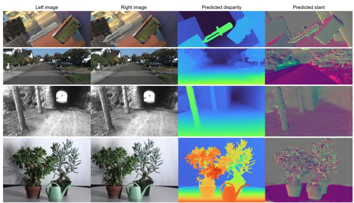
Figure 1: Example result of HITNet on the SceneFlow, KITTI, ETH3D and Middlebury datasets. Our approach predicts accurate depth with crisp edges. HITNet obtains state-of-art results on KITTI, ETH3D and Middlebury-v3 benchmarks.
图1:HITNet在SceneFlow、KITTI、ETH3D和Middlebury数据集上的示例结果。我们的方法能够预测出边缘清晰的准确深度。HITNet在KITTI、ETH3D和Middlebury - v3基准测试中取得了最先进的结果。
To summarize, our main contributions are:
综上所述,我们的主要贡献如下:
-
A fast multi-resolution initialization step that computes high resolution matches using learned features.
-
一个快速的多分辨率初始化步骤,使用学习到的特征计算高分辨率匹配。
-
An efficient 2D disparity propagation that makes use of slanted support windows with learned descriptors.
-
一种高效的二维视差传播方法,利用带有学习描述符的倾斜支持窗口。
-
State-of-art results in popular benchmarks using a fraction of the computation compared to other methods.
-
在流行的基准测试中取得了最先进的结果,与其他方法相比,计算量仅为其一小部分。
2. Related Work
2. 相关工作
Stereo matching has been an active field of research for decades [37, 44, 19]. Traditional methods utilize handcrafted schemes to find local correspondences [57, 22, 4, 21] and global optimization to exploit spatial context \(\left\lbrack {{14},{26},{27}}\right\rbrack\) . The run-time efficiency of most of these approaches are correlated with the size of the disparity space, which prevents real-time applications. Efficient algorithms \(\left\lbrack {{31},{35},5,3}\right\rbrack\) avoid searching the full disparity space by using patchmatch [1] and super-pixel [31] techniques. A family of machine learning based approaches, using random forest and decision trees, are able to establish correspondences quickly \(\left\lbrack {{10},{11},{12},{13}}\right\rbrack\) . However, these methods require either camera specific learning or post processing. Recently, deep learning brought big improvements to stereo matching. Early works trained siamese networks to extract patch-wise features or predict matching costs \(\left\lbrack {{36},{60},{58},{59}}\right\rbrack\) . End-to-end networks have been proposed to learn all steps jointly, yielding more accurate results [47, 38, 41, 48].
立体匹配几十年来一直是一个活跃的研究领域[37, 44, 19]。
- 传统方法利用手工设计的方案来寻找局部对应关系[57, 22, 4, 21],并使用全局优化来利用空间上下文\(\left\lbrack {{14},{26},{27}}\right\rbrack\)。大多数这些方法的运行时效率与视差空间的大小相关,这阻碍了实时应用。高效算法\(\left\lbrack {{31},{35},5,3}\right\rbrack\)通过使用块匹配[1]和超像素[31]技术避免搜索整个视差空间。
- 一类基于机器学习的方法,使用随机森林和决策树,能够快速建立对应关系\(\left\lbrack {{10},{11},{12},{13}}\right\rbrack\)。然而,这些方法要么需要特定相机的学习,要么需要后处理。
- 最近,深度学习给立体匹配带来了巨大的改进。早期的工作训练孪生网络来提取逐块特征或预测匹配成本\(\left\lbrack {{36},{60},{58},{59}}\right\rbrack\)。已经提出了端到端网络来联合学习所有步骤,从而得到更准确的结果[47, 38, 41, 48]。
A key component in modern architectures is a cost volume layer [24] (or correlation layer [23]), allowing the network to run per-pixel feature matching. To speed up computation, cascaded models \(\left\lbrack {{40},7,{33},{16},{54},{61}}\right\rbrack\) have been proposed to search in disparity space in a coarse-to-fine fashion. In particular, [40] uses multiple residual blocks to improve the current disparity estimate. The recent work [54] relies on a hierarchical cost volume, allowing the method to be trained on high resolution images and generate different resolutions on demand. All these methods rely on expensive cost-volume filtering operations using 3D convolutions [54] or multiple refinement layers [40], preventing real-time performance. Fast approaches \(\left\lbrack {{25},{62}}\right\rbrack\) down-sample the cost volume in spatial and disparity space and attempt to recover fine details by edge-aware upsampling layers. These methods show real-time performance but sacrifice accuracy especially for thin structures and edges since they are missing in the low-res initialization.
现代架构中的一个关键组件是代价体积层24,它允许网络进行逐像素特征匹配。
- 为了加速计算,已经提出了级联模型\(\left\lbrack {{40},7,{33},{16},{54},{61}}\right\rbrack\)以从粗到细的方式在视差空间中进行搜索。特别是,[40]使用多个残差块来改进当前的视差估计。
- 最近的工作[54]依赖于分层代价体积,允许该方法在高分辨率图像上进行训练,并按需生成不同分辨率的结果。所有这些方法都依赖于使用三维卷积[54]或多个细化层[40]的昂贵代价体积滤波操作,这阻碍了实时性能。
- 快速方法\(\left\lbrack {{25},{62}}\right\rbrack\)在空间和视差空间中对代价体积进行下采样,并尝试通过边缘感知上采样层恢复精细细节。这些方法显示出实时性能,但牺牲了准确性,特别是对于细结构和边缘,因为它们在低分辨率初始化中缺失。
Our method is inspired by classical stereo matching methods, which aim at propagating good sparse matches \(\left\lbrack {{12},{13},{52}}\right\rbrack\) . In particular, Tankovich et al. [52] proposed a hierarchical algorithm that makes use of slanted support windows to amortize the matching cost computation in tiles. Inspired by this work, we propose an end-to-end learning approach that overcomes the issues of hand-crafted algorithms, while maintaining computational efficiency.
我们的方法受到经典立体匹配方法的启发,这些方法旨在传播良好的稀疏匹配\(\left\lbrack {{12},{13},{52}}\right\rbrack\)。
- 特别是,Tankovich等人[52]提出了一种分层算法,利用倾斜支持窗口来平摊图像块中的匹配成本计算。
- 受这项工作的启发,我们提出了一种端到端学习方法,克服了手工设计算法的问题,同时保持了计算效率。
PWC-Net [50], although designed for optical flow estimation, is related to our approach. The method uses a low resolution cost volume with multiple refinement stages via image warps and local matching cost computations. Thereby following the classical pyramidal matching approach where a low resolution result gets hierarchically up-sampled and refined by initializing the current level with the previous level's solution. In contrast we propose a fast, multi-scale, high resolution initialization which is able to recover fine details that cannot be represented at low resolution. Finally, our refinement steps produce local slanted plane approximations, which are used to predict the final disparities, as opposed to standard bilinear warping and interpolation employed in [50].
PWC-Net [50] 虽然是为光流估计而设计的,但与我们的方法相关。
- 该方法使用低分辨率的代价体,并通过图像扭曲和局部匹配代价计算进行多个细化阶段。因此,它遵循经典的金字塔匹配方法,即低分辨率结果通过将当前层初始化为前一层的解进行分层上采样和细化。
- 相比之下,我们提出了一种快速、多尺度、高分辨率的初始化方法,能够恢复低分辨率下无法表示的精细细节。
- 最后,我们的细化步骤生成局部倾斜平面近似,用于预测最终视差,这与 [50] 中采用的标准双线性扭曲和插值方法不同。
3. Method
3. 方法
The design of HITNet, follows the principles of traditional stereo matching methods [44]. In particular, we observe that recent efficient methods rely on the three following steps: ① compact feature representations are extracted \(\left\lbrack {{12},{13}}\right\rbrack\) ; ② a high resolution disparity initialization step utilizes these features to retrieve feasible hypotheses; ③ an efficient propagation step refines the estimates using slanted support windows [52]. Motivated by these observations, we represent the disparity map as planar tiles at various resolutions and attach a learnable feature vector to each tile hypothesis (Sec. 3.1). This allows our network to learn which information about a small part of the disparity map is relevant to further improving the result. This can be interpreted as an efficient and sparse version of the learnable 3D cost volumes that have shown to be beneficial [24].
HITNet 的设计遵循传统立体匹配方法的原则 [44]。具体而言,我们发现最近的高效方法依赖于以下三个步骤:
- ① 提取紧凑的特征表示 \(\left\lbrack {{12},{13}}\right\rbrack\);
- ② 高分辨率视差初始化步骤利用这些特征来获取可行的假设;
- ③ 高效的传播步骤使用倾斜支持窗口来细化估计结果 [52]。
受这些观察结果的启发,我们将视差图表示为不同分辨率的平面块,并为每个块假设附加一个可学习的特征向量(第 3.1 节)。这使我们的网络能够学习视差图的一小部分信息对进一步改善结果的相关性。这可以被解释为可学习的 3D 代价体的一种高效且稀疏的版本,已证明这种版本是有益的 [24]。
The overall method is depicted in Fig. 2. Our feature extraction module relies on a very small U-Net [42], where the multi-resolution features of the decoder are used by the rest of the pipelines. These features encode multi-scale details of the image, similar to [7] (Sec. 3.2). Once the features are extracted, we initialize disparity maps as fronto parallel tiles at multiple resolutions. To do so, a matcher evaluates multiple hypotheses and selects the one with the lowest \({\ell }_{1}\) distance between left and right view feature. Additionally, a compact per-tile descriptor is computed using a small network (Sec. 3.3). The output of the initialization is then passed to a propagation stage, which acts similarly to the approximated Conditional Random Field solution used in \(\left\lbrack {{12},{52}}\right\rbrack\) . This stage hierarchically refines the tile hypotheses in an iterative fashion (Sec. 3.4).
整体方法如图 2 所示。
- 我们的特征提取模块依赖于一个非常小的 U-Net [42],解码器的多分辨率特征被管道的其余部分使用。这些特征对图像的多尺度细节进行编码,类似于 [7](第 3.2 节)。
- 一旦提取了特征,我们将视差图初始化为多个分辨率的前平行块。
- 为此,匹配器评估多个假设,并选择左右视图特征之间 \({\ell }_{1}\) 距离最小的假设。
- 此外,使用一个小网络计算每个块的紧凑描述符(第 3.3 节)。
- 初始化的输出然后传递到传播阶段,该阶段的作用类似于 \(\left\lbrack {{12},{52}}\right\rbrack\) 中使用的近似条件随机场解决方案。这个阶段以迭代的方式分层细化块假设(第 3.4 节)。

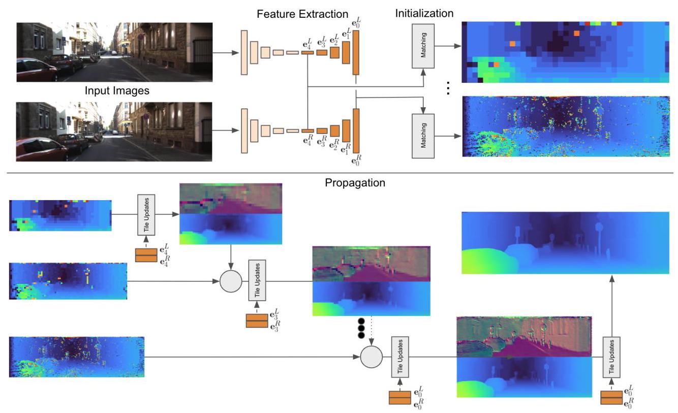
Figure 2: Overview of the proposed framework. (Top) A U-Net is used to extract features at multiple scales from left and right images. The initialization step is run on each scale of the extracted features. This step operates on tiles of \(4 \times 4\) feature regions and evaluates multiple disparity hypotheses. The disparity with the minimum cost is selected. (Bottom) The output of the initialization is then used at propagation stage to refine the predicted disparity hypotheses using slanted support windows.
图2:所提出框架的概述。(顶部)使用U-Net从左图像和右图像中提取多尺度特征。初始化步骤在提取的特征的每个尺度上运行。此步骤对\(4 \times 4\)特征区域的图块进行操作,并评估多个视差假设。选择成本最小的视差。(底部)初始化的输出随后在传播阶段用于使用倾斜支持窗口细化预测的视差假设。
3.1. Tile Hypothesis
3.1. 块假设
We define a tile hypothesis as a planar patch with a learnable feature attached to it. Concretely, it consists of a geometric part describing a slanted plane with the disparity \(d\) and the gradient of disparity in \(x\) and \(y\) directions \(\left( {{d}_{x},{d}_{y}}\right)\) , and a learnable part \(\mathbf{p}\) which we call tile feature descriptor. The hypothesis is therefore described as a vector which encodes a slanted 3D plane,
我们将块假设定义为一个附有可学习特征的平面块。具体来说,它由一个几何部分和一个可学习部分 \(\mathbf{p}\) 组成,几何部分描述了一个具有视差 \(d\) 以及视差在 \(x\) 和 \(y\) 方向上的梯度 \(\left( {{d}_{x},{d}_{y}}\right)\) 的倾斜平面,可学习部分我们称为块特征描述符。因此,该假设被描述为一个对倾斜 3D 平面进行编码的向量。
The tile feature descriptor is a learned representation of the tile which allows the network to attach additional information to the tile. This could for example be matching quality or local surface properties such as how planar the geometry actually is. We do not constrain this information and learned it end-to-end from the data instead.
块特征描述符是块的一种学习表示,它允许网络为块附加额外的信息。例如,这可能是匹配质量或局部表面属性,如几何形状实际上的平面程度。我们不限制这些信息,而是从数据中进行端到端的学习。
3.2. Feature Extractor
3.2. 特征提取器
The feature extractor provides a set of multi-scale feature maps \(\mathcal{E} = \left\{ {{\mathbf{e}}_{0},\ldots {\mathbf{e}}_{M}}\right\}\) that are used for initial matching and for warping in the propagation stage. We denote a feature map as \({\mathbf{e}}_{l}\) and an embedding vector \({\mathbf{e}}_{l, x, y}\) for locations \(x, y\) at resolution \(l \in 0,\ldots , M,0\) being the original image resolution and \(M\) denoting a \({2}^{M} \times {2}^{M}\) downsampled resolution. A single embedding vector \({\mathbf{e}}_{l, x, y}\) is composed of multiple feature channels. We implement the feature extractor \(\mathcal{E} = \mathcal{F}\left( {\mathbf{I};{\mathbf{\theta }}_{\mathcal{F}}}\right)\) as a U-Net like architecture [42,34], i.e. an encoder-decoder with skip connections, with learnable parameters \({\mathbf{\theta }}_{\mathcal{F}}\) . The network is composed of strided convolutions and transposed convolutions with leaky ReLUs as non-linearities. The set of feature maps \(\mathcal{E}\) that we use in the remainder of the network are the outputs of the upsam-pling part of the U-Net at all resolutions. This means that even the high resolution features do contain some amount of spatial context. In more details, one down-sampling block of the U-Net has a single \(3 \times 3\) convolution followed by a \(2 \times 2\) convolution with stride 2 . One up-sampling block applies \(2 \times 2\) stride 2 transpose convolutions to up-sample results of coarser U-Net resolution. Features are concatenated with skip-connection, and a \(1 \times 1\) convolution followed by a \(3 \times 3\) convolution are applied to merge the skipped and upsampled feature for the current resolution. Each upsam-pling block generates a feature map \({\mathbf{e}}_{l}\) , which is then used for downstream tasks and also further upsampled in the U-Net to generate a higher resolution feature map. We run the feature extractor on the left and the right image and obtain two multi-scale representations \({\mathcal{E}}^{L}\) and \({\mathcal{E}}^{R}\) .
特征提取器提供了一组多尺度特征图\(\mathcal{E} = \left\{ {{\mathbf{e}}_{0},\ldots {\mathbf{e}}_{M}}\right\}\),这些特征图用于初始匹配以及传播阶段的变形操作。我们将特征图表示为\({\mathbf{e}}_{l}\),将位置\(x, y\)在分辨率\(l \in 0,\ldots , M,0\)(原始图像分辨率)和\(M\)(表示\({2}^{M} \times {2}^{M}\)下采样分辨率)下的嵌入向量表示为\({\mathbf{e}}_{l, x, y}\)。单个嵌入向量\({\mathbf{e}}_{l, x, y}\)由多个特征通道组成。我们将特征提取器\(\mathcal{E} = \mathcal{F}\left( {\mathbf{I};{\mathbf{\theta }}_{\mathcal{F}}}\right)\)实现为类似U-Net的架构[42,34],即具有跳跃连接的编码器 - 解码器,其具有可学习参数\({\mathbf{\theta }}_{\mathcal{F}}\)。该网络由步幅卷积和转置卷积组成,使用带泄漏修正线性单元(Leaky ReLU)作为非线性激活函数。我们在网络其余部分使用的特征图集\(\mathcal{E}\)是U-Net上采样部分在所有分辨率下的输出。这意味着即使是高分辨率特征也包含一定量的空间上下文信息。
更详细地说,U-Net的一个下采样块包含一个\(3 \times 3\)卷积,后面跟着一个步幅为2的\(2 \times 2\)卷积。一个上采样块应用步幅为2的\(2 \times 2\)转置卷积来对上采样较粗U-Net分辨率的结果。特征通过跳跃连接进行拼接,然后应用一个\(1 \times 1\)卷积,接着是一个\(3 \times 3\)卷积,以合并当前分辨率下的跳跃特征和上采样特征。每个上采样块生成一个特征图\({\mathbf{e}}_{l}\),该特征图随后用于下游任务,并且还会在U-Net中进一步上采样以生成更高分辨率的特征图。我们在左图像和右图像上运行特征提取器,得到两个多尺度表示\({\mathcal{E}}^{L}\)和\({\mathcal{E}}^{R}\)。
3.3. Initialization
3.3. 初始化
The goal of the initialization is to extract an initial disparity \({d}^{\text{init }}\) and a feature vector \({\mathbf{p}}^{\text{init }}\) for each tile at various resolutions. The output of the initialization is fronto-parallel tile hypotheses of the form \({\mathbf{h}}^{\text{init }} = \left\lbrack {{d}^{\text{init }},0,0,{\mathbf{p}}^{\text{init }}}\right\rbrack\) .
初始化的目标是为不同分辨率下的每个图块提取初始视差\({d}^{\text{init }}\)和特征向量\({\mathbf{p}}^{\text{init }}\)。初始化的输出是形式为\({\mathbf{h}}^{\text{init }} = \left\lbrack {{d}^{\text{init }},0,0,{\mathbf{p}}^{\text{init }}}\right\rbrack\)的前平行图块假设。
Tile Disparity. In order to keep the initial disparity resolution high we use overlapping tiles along the \(x\) direction, i.e. the width, in the right (secondary) image but we still use non-overlapping tiles in the left (reference) image for efficient matching. To extract the tile features we run a \(4 \times 4\) convolution on each extracted feature map \({\mathbf{e}}_{l}\) . The strides for the left (reference) image and the right (secondary) image are different to facilitate the aforementioned overlapping tiles. For the left image we use strides of \(4 \times 4\) and for the right image we use strides of \(4 \times 1\) , which is crucial to maintain the full disparity resolution to maximize accuracy. This convolution is followed by a leaky ReLU and an MLP.
图块视差。为了保持初始视差分辨率较高,我们在右(辅助)图像中沿\(x\)方向(即宽度方向)使用重叠图块,但在左(参考)图像中仍然使用非重叠图块以进行高效匹配。为了提取图块特征,我们对每个提取的特征图\({\mathbf{e}}_{l}\)运行一个\(4 \times 4\)卷积。左(参考)图像和右(辅助)图像的步幅不同,以实现上述重叠图块。对于左图像,我们使用\(4 \times 4\)的步幅,对于右图像,我们使用\(4 \times 1\)的步幅,这对于保持完整的视差分辨率以最大化精度至关重要。此卷积之后是一个带泄漏修正线性单元(Leaky ReLU)和一个多层感知机(MLP)。
The output of this step will be a new set of feature maps \(\widetilde{\mathcal{E}} = \left\{ {{\widetilde{\mathbf{e}}}_{0},\ldots ,{\widetilde{\mathbf{e}}}_{M}}\right\}\) with per tile features \({\widetilde{\mathbf{e}}}_{l, x, y}\) . Note that the width of the feature maps in \({\widetilde{\mathcal{E}}}^{L}\) and \({\widetilde{\mathcal{E}}}^{R}\) are now different. The per-tile features are explicitly matched along the scan lines. We define the matching cost \(\varrho\) at location(x, y) and resolution \(l\) with disparity \(d\) as:
此步骤的输出将是一组新的特征图\(\widetilde{\mathcal{E}} = \left\{ {{\widetilde{\mathbf{e}}}_{0},\ldots ,{\widetilde{\mathbf{e}}}_{M}}\right\}\),其中包含每个图块的特征\({\widetilde{\mathbf{e}}}_{l, x, y}\)。请注意,\({\widetilde{\mathcal{E}}}^{L}\)和\({\widetilde{\mathcal{E}}}^{R}\)中特征图的宽度现在不同。每个图块的特征会沿着扫描线进行显式匹配。我们将位置(x, y)、分辨率\(l\)且视差为\(d\)时的匹配成本\(\varrho\)定义为:
The initial disparities are then computed as:
然后,初始视差计算如下:
for each(x, y)location and resolution \(l\) , where \(D\) is the maximal disparity that is considered. Note that despite the fact that the initialization stage exhaustively computes matches for all disparities there is no need to ever store the whole cost volume. At test time only the location of the best match needs to be extracted, which can be done very efficiently utilizing fast memory, e.g. shared memory on GPUs and a fused implementation in a single Op. Hence, there is no need to store and process a 3D cost volume.
对于每个(x, y)位置和分辨率\(l\),其中\(D\)是所考虑的最大视差。请注意,尽管初始化阶段会对所有视差进行详尽的匹配计算,但无需存储整个成本体。在测试时,只需提取最佳匹配的位置,这可以利用快速内存(例如GPU上的共享内存)并通过单个操作的融合实现来高效完成。因此,无需存储和处理三维成本体。
Tile Feature Descriptor. The initialization stage also predicts a feature description \({\mathbf{p}}_{l, x, y}^{\text{init }}\) for each(x, y)location and resolution \(l\) :
图块特征描述符。初始化阶段还会为每个(x, y)位置和分辨率\(l\)预测一个特征描述\({\mathbf{p}}_{l, x, y}^{\text{init }}\):
The features are based on the embedding vector of the reference image \({\widetilde{\mathbf{e}}}_{l, x, y}^{L}\) and the costs \(\varrho\) of the best matching disparity \({d}_{\text{init }}\) . We utilize a perceptron \(\mathcal{D}\) , with learnable weights \({\mathbf{\theta }}_{\mathcal{D}}\) , which is implemented with a \(1 \times 1\) convolution followed by a leaky ReLU. The input to the tile feature descriptor includes the matching costs \(\varrho \left( \cdot \right)\) , which allows the network to get a sense of the confidence of the match.
这些特征基于参考图像的嵌入向量\({\widetilde{\mathbf{e}}}_{l, x, y}^{L}\)和最佳匹配视差\({d}_{\text{init }}\)的成本\(\varrho\)。我们使用一个感知机\(\mathcal{D}\),其权重\({\mathbf{\theta }}_{\mathcal{D}}\)是可学习的,该感知机通过一个\(1 \times 1\)卷积层后接一个带泄漏的ReLU激活函数来实现。图块特征描述符的输入包括匹配成本\(\varrho \left( \cdot \right)\),这使网络能够了解匹配的置信度。
3.4. Propagation
3.4. 传播
The propagation step takes tile hypotheses as input and outputs refined tile hypotheses based on spatial propagation of information and fusion of information. It internally warps the features from the feature extraction stage from the right image (secondary) to the left image (reference) in order to predict highly accurate offsets to the input tiles. An additional confidence is predicted which allows for effective fusion between hypotheses coming from earlier propagation layers and from the initialization stage.
传播步骤将图块假设作为输入,并基于信息的空间传播和信息融合输出细化后的图块假设。它会在内部将特征提取阶段从右图像(辅助图像)提取的特征扭曲到左图像(参考图像),以便预测输入图块的高精度偏移。此外,还会预测一个置信度,这有助于在早期传播层和初始化阶段的假设之间进行有效融合。
Warping. The warping step computes the matching costs between the feature maps \({\mathbf{e}}_{l}^{L}\) and \({\mathbf{e}}_{l}^{R}\) at the feature resolution \(l\) associated to the tiles. This step is used to build a local cost volume around the current hypothesis. Each tile hypothesis is converted into a planar patch of size \(4 \times 4\) that it originally covered in the feature map. We denote the corresponding \(4 \times 4\) local disparity map as \({\mathbf{d}}^{\prime }\) with
扭曲。扭曲步骤计算与图块相关的特征分辨率\(l\)下特征图\({\mathbf{e}}_{l}^{L}\)和\({\mathbf{e}}_{l}^{R}\)之间的匹配成本。此步骤用于在当前假设周围构建局部成本体。每个图块假设会转换为一个大小为\(4 \times 4\)的平面块,该平面块最初覆盖特征图中的区域。我们将对应的\(4 \times 4\)局部视差图表示为\({\mathbf{d}}^{\prime }\),其中
for patch coordinates \(i, j \in \{ 0,\cdots ,3\}\) . The local disparities are then used to warp the features \({\mathbf{e}}_{l}^{R}\) from the right (secondary) image to the left (reference) image using linear interpolation along the scan lines. This results in a warped feature representation \({\mathbf{e}}_{l}^{{R}^{\prime }}\) which should be very similar to the corresponding features of the left (reference) image \({\mathbf{e}}^{L}\) if the local disparity maps \({\mathbf{d}}^{\prime }\) are accurate. Comparing the features of the reference(x, y)tile with the warped secondary tile we define the cost vector \(\mathbf{\phi }\left( {\mathbf{e},{\mathbf{d}}^{\prime }}\right) \in {\mathbb{R}}^{16}\) as:
对于块坐标\(i, j \in \{ 0,\cdots ,3\}\)。然后,使用沿扫描线的线性插值,将局部视差用于将右(辅助)图像的特征\({\mathbf{e}}_{l}^{R}\)扭曲到左(参考)图像。如果局部视差图\({\mathbf{d}}^{\prime }\)准确,这将得到一个扭曲后的特征表示\({\mathbf{e}}_{l}^{{R}^{\prime }}\),该表示应与左(参考)图像的对应特征\({\mathbf{e}}^{L}\)非常相似。通过比较参考(x, y)图块的特征与扭曲后的辅助图块的特征,我们将成本向量\(\mathbf{\phi }\left( {\mathbf{e},{\mathbf{d}}^{\prime }}\right) \in {\mathbb{R}}^{16}\)定义为:
where \({c}_{i, j} = {\begin{Vmatrix}{\mathbf{e}}_{l,{4x} + i,{4y} + j}^{L} - {\mathbf{e}}_{l,{4x} + i - {\mathbf{d}}^{\prime }{}_{i, j},{4y} + j}^{R}\end{Vmatrix}}_{1}\) .
其中 \({c}_{i, j} = {\begin{Vmatrix}{\mathbf{e}}_{l,{4x} + i,{4y} + j}^{L} - {\mathbf{e}}_{l,{4x} + i - {\mathbf{d}}^{\prime }{}_{i, j},{4y} + j}^{R}\end{Vmatrix}}_{1}\) 。
Tile Update Prediction. This step takes \(n\) tile hypotheses as input and predicts deltas for the tile hypotheses plus a scalar value \(w\) for each tile indicating how likely this tile is to be correct, i.e. a confidence measure. This mechanism is implemented as a CNN module \(\mathcal{U}\) , the convolutional architecture allows the network to see the tile hypotheses in a spatial neighborhood and hence is able to spatially propagate information. A key part of this step is that we augment the tile hypothesis with the matching costs \(\phi\) from the warping step. By doing this for a small neighborhood in disparity space we build up a local cost volume which allows the network to refine the tile hypotheses effectively. Concretely, we displace all the disparities in a tile by a constant offset of one disparity1in the positive and negative directions and compute the cost three times. Using this let a be the augmented tile hypothesis map for input tile map \(\mathbf{h}\) :
图块更新预测。此步骤将 \(n\) 个图块假设作为输入,并预测图块假设的增量,同时为每个图块预测一个标量值 \(w\) ,该值表示该图块正确的可能性,即置信度度量。此机制通过一个卷积神经网络(CNN)模块 \(\mathcal{U}\) 实现,卷积架构使网络能够观察到空间邻域内的图块假设,从而能够在空间上传播信息。此步骤的一个关键部分是,我们用来自变形步骤的匹配成本 \(\phi\) 来增强图块假设。通过在视差空间的一个小邻域内进行此操作,我们构建了一个局部成本体,使网络能够有效地细化图块假设。具体而言,我们将图块中的所有视差在正负方向上分别偏移一个视差单位的恒定偏移量,并计算三次成本。利用此方法,设 a 为输入图块映射 \(\mathbf{h}\) 的增强图块假设映射:
(7)
for a location(x, y)and resolution \(l\) , The CNN module \({\mathcal{U}}_{l}\) then predicts updates for each of the \(n\) tile hypothesis maps and additionally \({w}^{i} \in \mathbb{R}\) which represent the confidence of the tile hypotheses:
对于位置 (x, y) 和分辨率 \(l\) ,CNN 模块 \({\mathcal{U}}_{l}\) 随后为 \(n\) 个图块假设映射中的每一个预测更新,并额外预测 \({w}^{i} \in \mathbb{R}\) ,其表示图块假设的置信度:
The architecture of \(\mathcal{U}\) is implemented with residual blocks [20] but without batch normalization. Following [25] we use dilated convolutions to increase the receptive field. Before running a sequence of residual blocks with varying dilation factors we run a \(1 \times 1\) convolution followed by a leaky ReLU to decrease the number of feature channels. The update module is applied in a hierarchical iterative fashion (see Fig. 2). At the lowest resolution \(l = M\) we only have 1 tile hypothesis per location from the initialization stage, hence \(n = 1\) . We apply the tile updates by summing the input tile hypotheses and the deltas and upsample the tiles by a factor of 2 in each direction. Thereby, the disparity \(d\) is upsam-pled using the plane equation of the tile and the remaining parts of the tile hypothesis \({d}_{x},{d}_{y}\) and \(\mathbf{p}\) are upsampled using nearest neighbor sampling. At the next resolution \(M - 1\) we now have two hypotheses: the one from the initialization stage and the upsampled hypotheses from the lower resolution, hence \(n = 2\) . We utilize the \({w}^{i}\) to select the updated tile hypothesis with highest confidence for each location. We iterate this procedure until we reach the resolution 0 , which corresponds to tile size \(4 \times 4\) and full disparity resolution in all our experiments. To further refine the disparity map we use the winning hypothesis for the \(4 \times 4\) tiles and apply propagation module 3 times: for \(4 \times 4,2 \times 2,1 \times 1\) resolutions, using \(n = 1\) . The output at tile size \(1 \times 1\) is our final prediction. More details about the network architecture are provided in the supplementary material.
\(\mathcal{U}\) 的架构采用残差块 [20] 实现,但不进行批量归一化。遵循文献 [25] ,我们使用空洞卷积来增大感受野。在运行一系列具有不同膨胀因子的残差块之前,我们先运行一个 \(1 \times 1\) 卷积,然后接一个带泄漏修正线性单元(Leaky ReLU)以减少特征通道的数量。更新模块以分层迭代的方式应用(见图 2)。在最低分辨率 \(l = M\) 下,我们在初始化阶段每个位置只有 1 个图块假设,因此 \(n = 1\) 。我们通过将输入图块假设和增量相加来应用图块更新,并在每个方向上将图块上采样 2 倍。由此,视差 \(d\) 使用图块的平面方程进行上采样,图块假设的其余部分 \({d}_{x},{d}_{y}\) 和 \(\mathbf{p}\) 使用最近邻采样进行上采样。在下一个分辨率 \(M - 1\) 下,我们现在有两个假设:一个来自初始化阶段,另一个是来自较低分辨率的上采样假设,因此 \(n = 2\) 。我们利用 \({w}^{i}\) 为每个位置选择置信度最高的更新后的图块假设。我们迭代此过程,直到达到分辨率 0 ,在我们所有的实验中,这对应于图块大小 \(4 \times 4\) 和全视差分辨率。为了进一步细化视差图,我们使用 \(4 \times 4\) 图块的获胜假设,并应用传播模块 3 次:对于 \(4 \times 4,2 \times 2,1 \times 1\) 个分辨率,使用 \(n = 1\) 。图块大小为 \(1 \times 1\) 时的输出即为我们的最终预测。关于网络架构的更多细节在补充材料中提供。
4. Loss Functions
4. 损失函数
Our network is trained end-to-end with ground truth disparities \({d}^{\text{gt }}\) utilizing the losses described in the remainder of this section. The final loss is a sum of the losses over all the scales and pixels: \(\mathop{\sum }\limits_{{l, x, y}}{L}_{l}^{\text{init }} + {L}_{l}^{\text{prop }} + {L}_{l}^{\text{slant }} + {L}_{l}^{\mathrm{w}}\) .
我们的网络使用本节其余部分描述的损失函数,结合真实视差 \({d}^{\text{gt }}\) 进行端到端训练。最终损失是所有尺度和像素上的损失之和: \(\mathop{\sum }\limits_{{l, x, y}}{L}_{l}^{\text{init }} + {L}_{l}^{\text{prop }} + {L}_{l}^{\text{slant }} + {L}_{l}^{\mathrm{w}}\) 。
4.1. Initialization Loss
4.1. 初始化损失
Ground truth disparities are given with subpixel precision, however matching in initialization happens with integer disparities. Therefore we compute the matching cost for subpixel disparities using linear interpolation. The cost for subpixel disparities is then given as
真实视差以亚像素精度给出,然而初始化阶段的匹配是基于整数视差进行的。因此,我们使用线性插值计算亚像素视差的匹配成本。亚像素视差的成本随后表示为
where we dropped the \(l, x, y\) subscripts for clarity. To compute them at multiple resolutions we maxpool the ground truth disparity maps to downsample them to the required resolution. We aim at training the features \(\mathcal{E}\) to be such that the matching cost \(\psi\) is smallest at the ground truth disparity and larger everywhere else. To achieve this, we impose an \({\ell }_{1}\) contrastive loss [18]
为清晰起见,我们去掉了 \(l, x, y\) 下标。为了在多个分辨率下计算它们,我们对真实视差图进行最大池化操作,将其下采样到所需的分辨率。我们的目标是训练特征 \(\mathcal{E}\),使得匹配代价 \(\psi\) 在真实视差处最小,而在其他地方更大。为了实现这一点,我们引入了 \({\ell }_{1}\) 对比损失 [18]
where \(\beta > 0\) is a margin, \({d}^{\text{gt }}\) the ground truth disparity for a specific location and
其中 \(\beta > 0\) 是一个边界值,\({d}^{\text{gt }}\) 是特定位置的真实视差,
the disparity of the lowest cost non match for the same location. This cost pushes the ground truth cost toward 0 as well as the lowest cost non match toward a certain margin. In all our experiments we set the margin to \(\beta = 1\) . Similar contrastive losses have been used to learn the matching score in earlier deep learning based approaches to stereo matching \(\left\lbrack {{60},{36}}\right\rbrack\) . However, they either used a random non-matching location as negative sample or used all the non matching locations as negative samples, respectively.
以及同一位置的最低代价非匹配视差。这种代价将真实代价推向 0,同时将最低代价非匹配视差推向某个边界值。在我们所有的实验中,我们将边界值设置为 \(\beta = 1\)。类似的对比损失已在早期基于深度学习的立体匹配方法 \(\left\lbrack {{60},{36}}\right\rbrack\) 中用于学习匹配分数。然而,它们分别要么使用随机的非匹配位置作为负样本,要么使用所有非匹配位置作为负样本。
4.2. Propagation Loss
4.2. 传播损失
During propagation we impose a loss on the tile geometry \(d,{d}_{x},{d}_{y}\) and the tile confidence \(w\) . We use the ground truth disparity \({d}^{\text{gt }}\) and ground truth disparity gradients \({d}_{x}^{\text{gt }}\) and \({d}_{y}^{\mathrm{{gt}}}\) , which we compute by robustly fitting a plane to \({d}^{\mathrm{{gt}}}\) in a \(9 \times 9\) window centered at the pixel. In order to apply the loss on the tile geometry we first expand the tiles to a full resolution disparities \(\widehat{d}\) using the plane equation \(\left( {d,{d}_{x},{d}_{y}}\right)\) analogously to Eq. 5. The slant portion is also up-sampled to full resolution using nearest neighbor approach before slant loss is applied. We use the general robust loss function \(\rho \left( \cdot \right)\) from [2] which resembles a smooth \({\ell }_{1}\) loss, i.e., Huber loss. Additionally, we apply a truncation to the loss with threshold \(A\)
在传播过程中,我们对图块几何形状 \(d,{d}_{x},{d}_{y}\) 和图块置信度 \(w\) 施加损失。我们使用真实视差 \({d}^{\text{gt }}\) 和真实视差梯度 \({d}_{x}^{\text{gt }}\) 以及 \({d}_{y}^{\mathrm{{gt}}}\),这些是通过在以像素为中心的 \(9 \times 9\) 窗口内对 \({d}^{\mathrm{{gt}}}\) 进行稳健的平面拟合计算得到的。为了对图块几何形状施加损失,我们首先使用平面方程 \(\left( {d,{d}_{x},{d}_{y}}\right)\) 类似于公式 5 将图块扩展为全分辨率视差 \(\widehat{d}\)。在应用倾斜损失之前,倾斜部分也使用最近邻方法上采样到全分辨率。我们使用文献 [2] 中的通用稳健损失函数 \(\rho \left( \cdot \right)\),它类似于平滑的 \({\ell }_{1}\) 损失,即 Huber 损失。此外,我们对损失进行截断,阈值为 \(A\)
where \({d}^{\text{diff }} = {d}^{\text{gt }} - \widehat{d}\) . Further we impose a loss on the surface slant, as
其中 \({d}^{\text{diff }} = {d}^{\text{gt }} - \widehat{d}\)。此外,我们对表面倾斜施加损失,如下
where \(\chi\) is an indicator function which evaluates to 1 when the condition is satisfied and 0 otherwise. To supervise the confidence \(w\) we impose a loss which increases the confidence if the predicted hypothesis is closer than a threshold \({C}_{1}\) from the ground truth and decrease the confidence if the predicted hypothesis is further than a threshold \({C}_{2}\) away from the ground truth.
其中 \(\chi\) 是一个指示函数,当条件满足时取值为 1,否则取值为 0。为了监督置信度 \(w\),我们施加一个损失,如果预测假设与真实值的距离小于阈值 \({C}_{1}\),则增加置信度;如果预测假设与真实值的距离大于阈值 \({C}_{2}\),则降低置信度。
(14)
For all our experiments \(A = B = {C}_{1} = 1;{C}_{2} = {1.5}\) . For the last several levels, when only a single hypotheses is available, loss is applied to all pixels \(\left( {A = \infty }\right)\) .
在我们所有的实验中 \(A = B = {C}_{1} = 1;{C}_{2} = {1.5}\)。对于最后几个层级,当只有一个假设可用时,对所有像素 \(\left( {A = \infty }\right)\) 施加损失。
5. Experiments
5. 实验
We evaluate the proposed approach on popular benchmarks showing competitive results at a fraction of the computational time compared to other methods. We consider the following datasets: SceneFlow [38], KITTI 2012 [15], KITTI 2015 [39], ETH3D [45], Middlebury dataset V3 [43]. Following the standard evaluation settings we consider the two popular metrics: the End-Point-Error (EPE), which is the absolute distance in disparity space between the predicted output and the groundtruth; the \(x\) -pixels error, which is the percentage of pixels with disparity error greater than \(x\) . For the EPE computation on SceneFlow we adopt the same methodology of PSMNet [7], which excludes all the pixel with ground truth disparity bigger than 192 from the evaluation. Unless stated otherwise we use a HITNet with 5 levels, i.e. \(M = 4\) .
我们在流行的基准测试中评估了所提出的方法,与其他方法相比,在计算时间的一小部分内显示出具有竞争力的结果。我们考虑以下数据集:SceneFlow [38]、KITTI 2012 [15]、KITTI 2015 [39]、ETH3D [45]、Middlebury 数据集 V3 [43]。遵循标准评估设置,我们考虑两个流行的指标:端点误差(EPE),即预测输出与真实值在视差空间中的绝对距离;\(x\) 像素误差,即视差误差大于 \(x\) 的像素百分比。在 SceneFlow 上计算 EPE 时,我们采用与 PSMNet [7] 相同的方法,即从评估中排除所有真实视差大于 192 的像素。除非另有说明,我们使用具有 5 个层级的 HITNet,即 \(M = 4\)。
In this section we focus on comparisons with state-of-art on popular benchmarks, detailed ablation studies, run-time breakdown, cross-domain generalization and additional evaluations, are provided in the supplementary material. The trained models used for submission to benchmarks and evaluation scripts can be found at https://github.com/google-research/google-research/tree/master/hitnet
在本节中,我们专注于与流行基准测试中的最先进方法进行比较,详细的消融研究、运行时间分解、跨领域泛化和额外评估在补充材料中提供。用于提交到基准测试的训练模型和评估脚本可以在 https://github.com/google - research/google - research/tree/master/hitnet 找到。
5.1. Comparisons with State-of-the-art
5.1. 与最先进方法的比较
SceneFlow. On the synthetic dataset SceneFlow "final-pass" we achieve the remarkable End-Point-Error (EPE) of 0.36, which is \(2\mathrm{X}\) better than state-of-art at time of writing (see supplementary materials for details of \(\mathrm{L}\) and \(\mathrm{{XL}}\) versions). Representative competitors are reported in Tab. 1. The PSMNet algorithm [7] performs multi-scale feature extraction similarly to our method, but in contrast they use a more sophisticated pooling layer. Here we show that our architecture is more effective. Compared to GA-Net [61], we do not need complex message passing steps such as SGM. The results we obtain show that our strategy is also achieving a very similar inference. Finally, a representative fast method, StereoNet [25] is considered, which we consistently outperform. As result our method achieves the lowest EPE while still maintaining real-time performance. See Figure 3 for qualitative results.
场景流(SceneFlow) 在合成数据集SceneFlow “最终通道(final-pass)”上,我们实现了卓越的端点误差(End-Point-Error,EPE)为0.36,这比撰写本文时的最先进水平\(2\mathrm{X}\)还要好(有关\(\mathrm{L}\)和\(\mathrm{{XL}}\)版本的详细信息,请参阅补充材料)。表1中列出了具有代表性的竞争对手。PSMNet算法[7]与我们的方法类似,都进行多尺度特征提取,但不同的是,他们使用了更复杂的池化层。在这里,我们证明了我们的架构更有效。与GA-Net [61]相比,我们不需要像半全局匹配(SGM)这样复杂的消息传递步骤。我们获得的结果表明,我们的策略也能实现非常相似的推理。最后,考虑了一种具有代表性的快速方法StereoNet [25],我们始终优于该方法。因此,我们的方法在保持实时性能的同时,实现了最低的EPE。定性结果见图3。
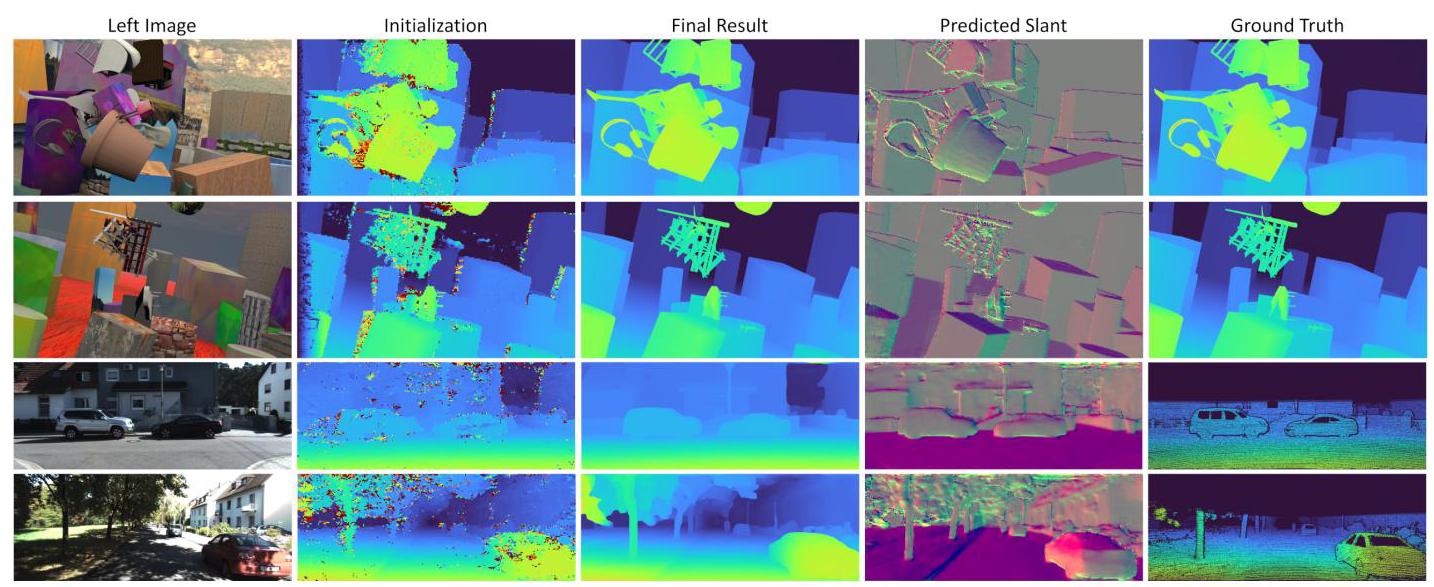
Figure 3: Qualitative results on SceneFlow and KITTI 2012. Note how the model is able to recover fine details, textureless regions and crisp edges.
图3:SceneFlow和KITTI 2012上的定性结果。请注意该模型如何能够恢复精细细节、无纹理区域和清晰边缘。
| Method | EPE px | Runtime s |
| HITNet XL | 0.36 | 0.114 |
| HITNet L | 0.43 | 0.054 |
| EdgeStereo [49] | 0.74 | 0.32 |
| LEAStereo [8] | 0.78 | 0.3 |
| GA-Net [61] | 0.84 | 1.6 |
| PSMNet [7] | 1.09 | 0.41 |
| StereoNet [25] | 1.1 | 0.015 |
Table 1: Comparisons with state-of-the-art methods on Scene Flow "finalpass" dataset, lower is better.
表1:在Scene Flow “最终通道(finalpass)”数据集上与最先进方法的比较,数值越低越好。
| Method | EPE px | Bad 1 | Bad 2 | Runtime |
| HITNet (ours) | 0.20 | 2.79 | 0.80 | 0.02 s |
| R-Stereo | 0.18 | 2.44 | 0.44 | 0.81 s |
| DN-CSS | 0.22 | 2.69 | 0.77 | 0.31 s |
| AdaStereo [48] | 0.26 | 3.41 | 0.74 | 0.40 s |
| Deep-Pruner [9] | 0.26 | 3.52 | 0.86 | 0.16 s |
| iResNet [33] | 0.24 | 3.68 | 1.00 | 0.20 s |
| Stereo-DRNet [6] | 0.27 | 4.46 | 0.83 | 0.33 s |
| PSMNet [7] | 0.33 | 5.02 | 1.09 | 0.54 s |
Table 2: Comparisons with state-of-the-art methods on ETH3D stereo dataset. For all metrics lower is better.
表2:在ETH3D立体数据集上与最先进方法的比较。所有指标都是数值越低越好。
Middlebury Stereo Dataset v3. We evaluated our method with multiple state-of-art approaches on the Middlebury stereo dataset v3, see Table 4 and the official benchmark website. \({}^{2}\) . As we can observe we outperform all the other end-to-end learning based approaches on most of the metrics, we rank among the top 10 when considering also hand-crafted approaches and in particular we rank first for bad 0.5 and A50, second for bad 1 and avgerr. In addition, we note that our average error is impacted by specifically one image, DjembL, which is due to the fact that we do not explicitly handle harsh lighting variations between input pairs. For visual results on the Middlebury datasets and details regarding the training procedure we refer the reader to the supplementary material.
Middlebury立体数据集v3 我们在Middlebury立体数据集v3上使用多种最先进的方法对我们的方法进行了评估,见表4和官方基准网站\({}^{2}\)。正如我们所观察到的,在大多数指标上,我们优于所有其他基于端到端学习的方法;当同时考虑手工制作的方法时,我们排名前10,特别是在坏点率0.5(bad 0.5)和A50指标上排名第一,在坏点率1(bad 1)和平均误差(avgerr)指标上排名第二。此外,我们注意到我们的平均误差特别受到一张图像DjembL的影响,这是因为我们没有明确处理输入图像对之间的强烈光照变化。关于Middlebury数据集的视觉结果和训练过程的详细信息,请参考补充材料。
ETH3D two view stereo. We evaluated our method with multiple state-of-art approaches on the ETH3D dataset, see Tab. 2. At time of submission to benchmark, HITNet ranks \({1}^{\text{st }} - {4}^{\text{rd }}\) on all the metrics published on the website. In particular, our method ranks \({1}^{\text{nd }}\) on the following metrics: bad 0.5, bad 4, average error, rms error, 50% quantile, 90% quantile: this shows that HITNet is resilient to the particular measurement chosen, whereas competitive approaches exhibits substantial differences when different metrics are selected. See the submission website for details. \({}^{3}\) .
ETH3D双视图立体。我们在ETH3D数据集上使用多种最先进的方法对我们的方法进行了评估,见表2。在提交基准测试时,HITNet在网站上公布的所有指标上排名\({1}^{\text{st }} - {4}^{\text{rd }}\)。特别是,我们的方法在以下指标上排名\({1}^{\text{nd }}\):坏点率0.5(bad 0.5)、坏点率4(bad 4)、平均误差、均方根误差、50%分位数、90%分位数:这表明HITNet对所选的特定测量指标具有鲁棒性,而竞争方法在选择不同指标时表现出显著差异。详细信息请参阅提交网站\({}^{3}\)。
KITTI 2012 and 2015. At time of writing, among the published methods faster than \({100}\mathrm{{ms}},\mathrm{{HITNetranks}}\# 1\) on KITTI 2012 and 2015 benchmarks. Compared to other state-of-the-art stereo matchers (see Tab. 3), our approach
KITTI 2012和2015。在撰写本文时,在KITTI 2012和2015基准测试中,在比\({100}\mathrm{{ms}},\mathrm{{HITNetranks}}\# 1\)更快的已发表方法中。与其他最先进的立体匹配器相比(见表3),我们的方法
\({}^{2}\) See "HITNet" entry on the official dataset website.
\({}^{2}\) 请参阅官方数据集网站上的“HITNet”条目。
\({}^{3}\) See the ETH3D Website at https://www.eth3d.net/low_res_two_view for the complete metrics.
\({}^{3}\) 请访问https://www.eth3d.net/low_res_two_view上的ETH3D网站获取完整指标。
| KITTI 2012 [15] | KITTI 2015 [39] | |||||||||
| Method | 2-noc | 2-all | 3-noc | 3-all | EPE noc | EPE all | D1-bg | D1-fg | D1-all | Run-time |
| HITNet (ours) | 2.00 | 2.65 | 1.41 | 1.89 | 0.4 | 0.5 | 1.74 | 3.20 | 1.98 | 0.02s |
| LEAStereo [8] | 1.90 | 2.39 | 1.13 | 1.45 | 0.4 | 0.5 | 1.40 | 2.91 | 1.65 | 0.3s |
| GANet-deep [61] | 1.89 | 2.50 | 1.19 | 1.6 | 0.4 | 0.5 | 1.48 | 3.46 | 1.81 | 1.8s |
| EdgeStereo-V2 [49] | 2.32 | 2.88 | 1.46 | 1.83 | 0.4 | 0.5 | 1.84 | 3.30 | 2.08 | 0.32s |
| GC-Net [24] | 2.71 | 3.46 | 1.77 | 2.30 | 0.6 | 0.7 | 2.21 | 6.16 | 2.87 | 0.9s |
| SGM-Net [46] | 3.60 | 5.15 | 2.29 | 3.50 | 0.7 | 0.9 | 2.66 | 8.64 | 3.66 | 67s |
| ESMNet [17] | 3.65 | 4.30 | 2.08 | 2.53 | 0.6 | 0.7 | 2.57 | 4.86 | 2.95 | 0.06s |
| MC-CNN-acrt [60] | 3.90 | 5.45 | 2.09 | 3.22 | 0.6 | 0.7 | 2.89 | 8.88 | 3.89 | 67s |
| RTSNet [29] | 3.98 | 4.61 | 2.43 | 2.90 | 0.7 | 0.7 | 2.86 | 6.19 | 3.41 | 0.02s |
| Fast DS-CS [56] | 4.54 | 5.34 | 2.61 | 3.20 | 0.7 | 0.8 | 2.83 | 4.31 | 3.08 | 0.02s |
| StereoNet [25] | 4.91 | 6.02 | - | - | 0.8 | 0.9 | 4.30 | 7.45 | 4.83 | 0.015s |
Table 3: Quantitative evaluation on KITTI 2012 and KITTI 2015. For KITTI 2012 we report the percentage of pixels with error bigger than \(x\) disparities in both non-occluded (x-noc) and all regions (x-all), as well as the overall EPE in both non occluded (EPE-noc) and all the pixels (EPE-all). For KITTI 2015 We report the percentage of pixels with error bigger than 1 disparity in background regions (bg), foreground areas (fg), and all.
表3:KITTI 2012和KITTI 2015上的定量评估。对于KITTI 2012,我们报告了在非遮挡区域(x-noc)和所有区域(x-all)中误差大于\(x\)视差的像素百分比,以及非遮挡区域(EPE-noc)和所有像素(EPE-all)的总体EPE。对于KITTI 2015,我们报告了背景区域(bg)、前景区域(fg)和所有区域中误差大于1视差的像素百分比。
| Method | RMS | AvgErr | Bad 0.5 | Bad 1.0 | Bad 2.0 | Bad 4.0 | A50 | Run-time |
| HITNet (ours) | 9.97 | 1.71 | 34.2 | 13.3 | 6.46 | 3.81 | 0.40 | 0.14 s |
| LEAStereo [8] | 8.11 | 1.43 | 49.5 | 20.8 | 7.15 | 2.75 | 0.53 | 2.9 s |
| NOSS-ROB [30] | 12.2 | 2.08 | 38.2 | 13.2 | 5.01 | 3.46 | 0.42 | 662s (CPU) |
| LocalExp [51] | 13.4 | 2.24 | 38.7 | 13.9 | 5.43 | 3.69 | 0.43 | 881s (CPU) |
| CRLE [53] | 13.6 | 2.25 | 38.1 | 13.4 | 5.75 | 3.90 | 0.42 | 1589s (CPU) |
| HSM [54] | 10.3 | 2.07 | 50.7 | 24.6 | 10.2 | 4.83 | 0.56 | 0.51 s |
| MC-CNN [60] | 21.3 | 3.82 | 40.7 | 17.1 | 8.08 | 4.91 | 0.45 | 150 s |
| EdgeStereo [49] | 9.84 | 2.67 | 55.6 | 32.4 | 18.7 | 10.8 | 0.72 | 0.35 s |
Table 4: Comparisons with state-of-the-art methods on Middlebury V3 dataset. For all metrics lower is better.
表4:在Middlebury V3数据集上与最先进方法的比较。所有指标都是数值越低越好。
compares favorably to GC-Net [24], [40] and many others. Recent methods such as GA-Net [61] and HSM [54] are obtaining slightly better metrics, although they require 1.8 and 0.15 seconds respectively. Note also that HSM [54] has been trained with additional external high resolution data. Similarly, GA-Net [61] is pre-trained on SceneFlow and fine-tuned on KITTI benchmarks, whereas our approach is fully trained on the small data available on KITTI. Compared to fast methods such as StereoNet [25] and RTSNet [29], our method consistently outperforms them by a considerable margin, showing that it can be employed in latency critical scenarios without sacrificing accuracy. \({}^{4}\) .
与GC - Net [24]、[40]等许多方法相比,表现更优。诸如GA - Net [61]和HSM [54]等近期方法在指标上略有优势,不过它们分别需要1.8秒和0.15秒。还需注意的是,HSM [54]是使用额外的外部高分辨率数据进行训练的。同样,GA - Net [61]在SceneFlow上进行预训练,并在KITTI基准测试上进行微调,而我们的方法是完全在KITTI上可用的少量数据上进行训练的。与StereoNet [25]和RTSNet [29]等快速方法相比,我们的方法始终大幅超越它们,这表明它可以在对延迟要求严格的场景中使用,且不牺牲准确性。\({}^{4}\) 。
6. Conclusion
6. 结论
We presented HITNet, a real-time end-to-end architecture for accurate stereo matching. We presented a fast initialization step that is able to compute high resolution matches using learned features very efficiently. These tile initializations are then fused using propagation and fusion steps. The use of slanted support windows with learned descriptors provides additional accuracy. We presented state-of-the art accuracy on multiple commonly used benchmarks. A limitation of our algorithm is that it needs to be trained on a dataset with ground truth depth. To address this in the future we are planning to investigate self-supervised methods and self-distillation methods to further increase the accuracy and decrease the amount of training data that is required. A limitation of our experiments is that different datasets are trained on separately and use slightly different model architectures. To address this in the future, a single experiment is required that aligns with Robust Vision Challenge requirements.
我们提出了HITNet,这是一种用于精确立体匹配的实时端到端架构。我们提出了一个快速初始化步骤,该步骤能够利用学习到的特征非常高效地计算高分辨率匹配。然后通过传播和融合步骤将这些分块初始化结果进行融合。使用带有学习到的描述符的倾斜支持窗口可进一步提高准确性。我们在多个常用基准测试中展现了最先进的准确性。我们算法的一个局限性在于它需要在具有真实深度数据的数据集上进行训练。为了在未来解决这个问题,我们计划研究自监督方法和自蒸馏方法,以进一步提高准确性并减少所需的训练数据量。我们实验的一个局限性在于不同的数据集是分开训练的,并且使用了略有不同的模型架构。为了在未来解决这个问题,需要进行一个符合鲁棒视觉挑战要求的单一实验。
Acknowledgements. We would like to thank Shahram Izadi for support and enabling of this project.
致谢。我们要感谢Shahram Izadi对本项目的支持和促成。
References
参考文献
[1] Connelly Barnes, Eli Shechtman, Adam Finkelstein, and Dan B Goldman. Patchmatch: A randomized correspondence algorithm for structural image editing. ACM Transactions on Graphics (ToG), 2009. 2
[1] Connelly Barnes、Eli Shechtman、Adam Finkelstein和Dan B Goldman。Patchmatch:一种用于结构图像编辑的随机对应算法。《ACM图形学汇刊》(ACM Transactions on Graphics,ToG),2009年。2
\({}^{4}\) See the KITTI Website at http://www.cvlibs.net/datasets/kitti/eval_stereo.php for the complete metrics.
\({}^{4}\) 完整指标请见KITTI网站:http://www.cvlibs.net/datasets/kitti/eval_stereo.php 。
[2] Jonathan T Barron. A general and adaptive robust loss function. In IEEE Conference on Computer Vision and Pattern Recognition (CVPR), 2019. 6
[2] Jonathan T Barron。一种通用且自适应的鲁棒损失函数。《电气与电子工程师协会计算机视觉与模式识别会议》(IEEE Conference on Computer Vision and Pattern Recognition,CVPR),2019年。6
[3] Frederic Besse, Carsten Rother, Andrew Fitzgibbon, and Jan Kautz. Pmbp: Patchmatch belief propagation for correspondence field estimation. International Journal of Computer Vision (IJCV), 2014. 2
[3] Frederic Besse、Carsten Rother、Andrew Fitzgibbon和Jan Kautz。Pmbp:用于对应场估计的Patchmatch置信传播算法。《国际计算机视觉杂志》(International Journal of Computer Vision,IJCV),2014年。2
[4] Michael Bleyer and Margrit Gelautz. Simple but effective tree structures for dynamic programming-based stereo matching. In International Conference on Computer Vision Theory and Applications (VISAPP), 2008. 2
[4] Michael Bleyer和Margrit Gelautz。基于动态规划的立体匹配的简单而有效的树结构。《计算机视觉理论与应用国际会议》(International Conference on Computer Vision Theory and Applications,VISAPP),2008年。2
[5] Michael Bleyer, Christoph Rhemann, and Carsten Rother. Patchmatch stereo-stereo matching with slanted support windows. In British Machine Vision Conference (BMVC), 2011. 2
[5] Michael Bleyer、Christoph Rhemann和Carsten Rother。使用倾斜支持窗口的Patchmatch立体匹配算法。《英国机器视觉会议》(British Machine Vision Conference,BMVC),2011年。2
[6] Rohan Chabra, Julian Straub, Christopher Sweeney, Richard Newcombe, and Henry Fuchs. StereoDRNet: Dilated residual stereonet. In IEEE Conference on Computer Vision and Pattern Recognition, 2019. 7, 17
[6] Rohan Chabra、Julian Straub、Christopher Sweeney、Richard Newcombe和Henry Fuchs。StereoDRNet:扩张残差立体网络。《电气与电子工程师协会计算机视觉与模式识别会议》,2019年。7, 17
[7] Jia-Ren Chang and Yong-Sheng Chen. Pyramid stereo matching network. In IEEE Conference on Computer Vision and Pattern Recognition (CVPR), 2018. 3, 6, 7, 15, 17
[7] Jia - Ren Chang和Yong - Sheng Chen。金字塔立体匹配网络。《电气与电子工程师协会计算机视觉与模式识别会议》(IEEE Conference on Computer Vision and Pattern Recognition,CVPR),2018年。3, 6, 7, 15, 17
[8] Xuelian Cheng, Yiran Zhong, Mehrtash Harandi, Yuchao Dai, Xiaojun Chang, Tom Drummond, Hongdong Li, and Zongyuan Ge. Hierarchical neural architecture search for deep stereo matching. In NIPS, 2020. 7, 8, 17
[8] Xuelian Cheng、Yiran Zhong、Mehrtash Harandi、Yuchao Dai、Xiaojun Chang、Tom Drummond、Hongdong Li和Zongyuan Ge。用于深度立体匹配的分层神经架构搜索。《神经信息处理系统大会》(NIPS),2020年。7, 8, 17
[9] Shivam Duggal, Shenlong Wang, Wei-Chiu Ma, Rui Hu, and Raquel Urtasun. Deeppruner: Learning efficient stereo matching via differentiable patchmatch. 2019 IEEE/CVF International Conference on Computer Vision (ICCV), pages 4383-4392, 2019. 7
[9] Shivam Duggal、Shenlong Wang、Wei - Chiu Ma、Rui Hu和Raquel Urtasun。Deeppruner:通过可微Patchmatch学习高效立体匹配。《2019年电气与电子工程师协会/计算机视觉基金会国际计算机视觉会议》(2019 IEEE/CVF International Conference on Computer Vision,ICCV),第4383 - 4392页,2019年。7
[10] S. R. Fanello, C. Keskin, S. Izadi, P. Kohli, D. Kim, D. Sweeney, A. Criminisi, J. Shotton, S.B. Kang, and T. Paek. Learning to be a depth camera for close-range human capture and interaction. Transaction On Graphics (TOG), 2014. 2
[10] S. R. Fanello、C. Keskin、S. Izadi、P. Kohli、D. Kim、D. Sweeney、A. Criminisi、J. Shotton、S.B. Kang和T. Paek。学习成为用于近距离人体捕捉和交互的深度相机。《图形学汇刊》(Transaction On Graphics,TOG),2014年。2
[11] S. R. Fanello, C. Rhemann, V. Tankovich, A. Kowdle, S. Orts Escolano, D. Kim, and S. Izadi. Hyperdepth: Learning depth from structured light without matching. In IEEE Conference on Computer Vision and Pattern Recognition (CVPR), 2016. 2
[11] S. R. 法内洛(S. R. Fanello)、C. 雷曼(C. Rhemann)、V. 坦科维奇(V. Tankovich)、A. 科德尔(A. Kowdle)、S. 奥尔茨·埃斯科拉诺(S. Orts Escolano)、D. 金(D. Kim)和 S. 伊扎迪(S. Izadi)。超深度:无需匹配从结构光中学习深度。见《电气与电子工程师协会计算机视觉与模式识别会议论文集》(IEEE Conference on Computer Vision and Pattern Recognition,CVPR),2016 年。2
[12] Sean Ryan Fanello, Julien Valentin, Adarsh Kowdle, Christoph Rhemann, Vladimir Tankovich, Carlo Ciliberto, Philip Davidson, and Shahram Izadi. Low compute and fully parallel computer vision with hashmatch. Inernational Conference on Computer Vision (ICCV), 2017. 2, 3
[12] 肖恩·瑞安·法内洛(Sean Ryan Fanello)、朱利安·瓦伦丁(Julien Valentin)、阿达什·科德尔(Adarsh Kowdle)、克里斯托夫·雷曼(Christoph Rhemann)、弗拉基米尔·坦科维奇(Vladimir Tankovich)、卡罗·奇利贝托(Carlo Ciliberto)、菲利普·戴维森(Philip Davidson)和沙赫拉姆·伊扎迪(Shahram Izadi)。基于哈希匹配的低计算量全并行计算机视觉。见《国际计算机视觉会议论文集》(Inernational Conference on Computer Vision,ICCV),2017 年。2, 3
[13] Sean Ryan Fanello, Julien Valentin, Christoph Rhemann, Adarsh Kowdle, Vladimir Tankovich, Philip Davidson, and Shahram Izadi. Ultrastereo: Efficient learning-based matching for active stereo systems. In IEEE Conference on Computer Vision and Pattern Recognition (CVPR), 2017. 2, 3
[13] 肖恩·瑞安·法内洛(Sean Ryan Fanello)、朱利安·瓦伦丁(Julien Valentin)、克里斯托夫·雷曼(Christoph Rhemann)、阿达什·科德尔(Adarsh Kowdle)、弗拉基米尔·坦科维奇(Vladimir Tankovich)、菲利普·戴维森(Philip Davidson)和沙赫拉姆·伊扎迪(Shahram Izadi)。超立体视觉:基于高效学习的主动立体视觉系统匹配方法。见《电气与电子工程师协会计算机视觉与模式识别会议论文集》(IEEE Conference on Computer Vision and Pattern Recognition,CVPR),2017 年。2, 3
[14] Pedro F Felzenszwalb and Daniel P Huttenlocher. Efficient belief propagation for early vision. International journal of computer vision (IJCV), 2006. 2
[14] 佩德罗·F·费尔曾斯瓦尔布(Pedro F Felzenszwalb)和丹尼尔·P·胡滕洛赫尔(Daniel P Huttenlocher)。早期视觉中的高效置信度传播。《国际计算机视觉杂志》(International journal of computer vision,IJCV),2006 年。2
[15] Andreas Geiger, Philip Lenz, and Raquel Urtasun. Are we ready for autonomous driving? the kitti vision benchmark suite. In IEEE Conference on Computer Vision and Pattern Recognition (CVPR), 2012. 6, 8, 15
[15] 安德烈亚斯·盖格(Andreas Geiger)、菲利普·伦茨(Philip Lenz)和拉奎尔·乌尔塔松(Raquel Urtasun)。我们准备好自动驾驶了吗?基蒂视觉基准套件。见《电气与电子工程师协会计算机视觉与模式识别会议论文集》(IEEE Conference on Computer Vision and Pattern Recognition,CVPR),2012 年。6, 8, 15
[16] Spyros Gidaris and Nikos Komodakis. Detect, replace, refine: Deep structured prediction for pixel wise labeling. In IEEE Conference on Computer Vision and Pattern Recognition (CVPR), 2017. 3
[16] 斯皮罗斯·吉达里斯(Spyros Gidaris)和尼科斯·科莫达基斯(Nikos Komodakis)。检测、替换、细化:用于逐像素标注的深度结构化预测。见《电气与电子工程师协会计算机视觉与模式识别会议论文集》(IEEE Conference on Computer Vision and Pattern Recognition,CVPR),2017 年。3
[17] Chenggang Guo, Dongyi Chen, and Zhiqi Huang. Learning efficient stereo matching network with depth discontinuity aware super-resolution. IEEE Access, 2019. 8
[17] 郭成刚、陈东毅和黄志奇。具有深度不连续感知超分辨率的高效立体匹配网络学习。《IEEE接入》,2019年,第8期
[18] Raia Hadsell, Sumit Chopra, and Yann LeCun. Dimensionality reduction by learning an invariant mapping. In IEEE Computer Society Conference on Computer Vision and Pattern Recognition (CVPR), 2006. 6
[18] 拉亚·哈德塞尔、苏米特·乔普拉和扬·勒昆。通过学习不变映射进行降维。见《IEEE计算机协会计算机视觉与模式识别会议(CVPR)》,2006年,第6期
[19] Rostam Affendi Hamzah and Haidi Ibrahim. Literature survey on stereo vision disparity map algorithms. Journal of Sensors, 2016. 2
[19] 罗斯塔姆·阿芬迪·哈姆扎和海迪·易卜拉欣。立体视觉视差图算法的文献综述。《传感器学报》,2016年,第2期
[20] Kaiming He, Xiangyu Zhang, Shaoqing Ren, and Jian Sun. Deep residual learning for image recognition. In IEEE conference on computer vision and pattern recognition (CVPR), 2016. 5
[20] 何恺明、张祥雨、任少卿和孙剑。用于图像识别的深度残差学习。见《IEEE计算机视觉与模式识别会议(CVPR)》,2016年,第5期
[21] Heiko Hirschmuller. Stereo processing by semiglobal matching and mutual information. IEEE Transactions on pattern analysis and machine intelligence (TPAMI), 2008. 2
[21] 海科·赫希米勒。基于半全局匹配和互信息的立体处理。《IEEE模式分析与机器智能汇刊(TPAMI)》,2008年,第2期
[22] Asmaa Hosni, Christoph Rhemann, Michael Bleyer, Carsten Rother, and Margrit Gelautz. Fast cost-volume filtering for visual correspondence and beyond. IEEE Transactions on Pattern Analysis and Machine Intelligence (TPAMI), 2013. 2
[22] 阿斯玛·霍斯尼、克里斯托夫·雷曼、迈克尔·布莱尔、卡斯滕·罗瑟和玛格丽特·格拉茨。用于视觉对应及其他方面的快速代价体滤波。《IEEE模式分析与机器智能汇刊(TPAMI)》,2013年,第2期
[23] Eddy Ilg, Nikolaus Mayer, Tonmoy Saikia, Margret Keuper, Alexey Dosovitskiy, and Thomas Brox. Flownet 2.0: Evolution of optical flow estimation with deep networks. In IEEE Conference on Computer Vision and Pattern Recognition (CVPR), 2017. 3
[23] 埃迪·伊尔格、尼古劳斯·迈尔、托莫伊·赛凯亚、玛格丽特·库珀、阿列克谢·多索维茨基和托马斯·布罗克斯。FlowNet 2.0:基于深度网络的光流估计的演进。见《IEEE计算机视觉与模式识别会议(CVPR)》,2017年,第3期
[24] Alex Kendall, Hayk Martirosyan, Saumitro Dasgupta, Peter Henry, Ryan Kennedy, Abraham Bachrach, and Adam Bry. End-to-end learning of geometry and context for deep stereo regression. In IEEE International Conference on Computer Vision (ICCV), 2017. 2, 3, 8, 13, 17
[24] 亚历克斯·肯德尔、海克·马尔蒂罗相、绍米特罗·达斯古普塔、彼得·亨利、瑞安·肯尼迪、亚伯拉罕·巴赫拉赫和亚当·布赖。用于深度立体回归的几何与上下文的端到端学习。见《IEEE国际计算机视觉会议(ICCV)》,2017年,第2、3、8、13、17期
[25] Sameh Khamis, Sean Fanello, Christoph Rhemann, Adarsh Kowdle, Julien Valentin, and Shahram Izadi. StereoNet: Guided hierarchical refinement for edge-aware depth prediction. In European Conference on Computer Vision (ECCV), 2018.2,3,5,7,8
[25] 萨米·哈米斯、肖恩·法内洛、克里斯托夫·雷曼、阿达什·科德尔、朱利安·瓦伦丁和沙赫拉姆·伊扎迪。StereoNet:用于边缘感知深度预测的引导式分层细化。见《欧洲计算机视觉会议(ECCV)》,2018年,第2、3、5、7、8期
[26] Andreas Klaus, Mario Sormann, and Konrad Karner. Segment-based stereo matching using belief propagation and a self-adapting dissimilarity measure. In International Conference on Pattern Recognition (ICPR), 2006. 2
[26] 安德烈亚斯·克劳斯、马里奥·索尔曼和康拉德·卡纳。基于分割的立体匹配,使用置信传播和自适应不相似度度量。见《国际模式识别会议(ICPR)》,2006年,第2期
[27] Vladimir Kolmogorov and Ramin Zabih. Computing visual correspondence with occlusions using graph cuts. In International Conference on Computer Vision (ICCV), 2001. 2
[27] 弗拉基米尔·科尔莫戈罗夫和拉明·扎比。使用图割计算存在遮挡情况下的视觉对应。见《国际计算机视觉会议(ICCV)》,2001年,第2期
[28] Adarsh Kowdle, Christoph Rhemann, Sean Fanello, Andrea Tagliasacchi, Jon Taylor, Philip Davidson, Mingsong Dou, Kaiwen Guo, Cem Keskin, Sameh Khamis, David Kim, Danhang Tang, Vladimir Tankovich, Julien Valentin, and Shahram Izadi. The need 4 speed in real-time dense visual tracking. Transaction On Graphics (TOG), 2018. 2
[28] 阿达什·科德尔、克里斯托夫·雷曼、肖恩·法内洛、安德里亚·塔利亚萨基、乔恩·泰勒、菲利普·戴维森、窦明松、郭凯文、塞姆·凯斯金、萨米·哈米斯、大卫·金、唐丹航、弗拉基米尔·坦科维奇、朱利安·瓦伦丁和沙赫拉姆·伊扎迪。实时密集视觉跟踪对速度的需求。《图形学汇刊(TOG)》,2018年,第2期
[29] H. Lee and Y. Shin. Real-time stereo matching network with high accuracy. In IEEE International Conference on Image Processing (ICIP), 2019. 8, 13
[29] 李H和申Y。高精度实时立体匹配网络。见《IEEE国际图像处理会议(ICIP)》,2019年,第8、13期
[30] Jie Li, Penglei Ji, and Xinguo Liu. Superpixel alpha-expansion and normal adjustment for stereo matching. In CAD/Graphics 2019, 2019. 8
[30] 李杰、姬朋磊和刘新国。用于立体匹配的超像素α扩展和法线调整。见《2019年计算机辅助设计与图形学会议(CAD/Graphics 2019)》,2019年,第8期
[31] Yu Li, Dongbo Min, Michael S Brown, Minh N Do, and Jiangbo Lu. SPM-BP: Sped-up patchmatch belief propagation for continuous mrfs. In IEEE International Conference on Computer Vision (ICCV), 2015. 2
[31] 李钰、闵东波、迈克尔·S·布朗、闵N·多和卢江波。SPM - BP:用于连续马尔可夫随机场的加速块匹配置信传播。见《IEEE国际计算机视觉会议(ICCV)》,2015年,第2期
[32] Zhengfa Liang, Yiliu Feng, Yulan Guo, Hengzhu Liu, Wei Chen, Linbo Qiao, Li Zhou, and Jianfeng Zhang. Learning for disparity estimation through feature constancy. 2018. 15
[32] 梁正发、冯一柳、郭玉兰、刘恒柱、陈炜、乔林波、周莉和张剑锋。通过特征恒常性进行视差估计学习。2018年,第15期
[33] Zhengfa Liang, Yiliu Feng, Yulan Guo, Hengzhu Liu, Linbo Qiao, Wei Chen, Li Zhou, and Jianfeng Zhang. Learning for disparity estimation through feature constancy. 2017. 3, 7
[33] 梁正发、冯一柳、郭玉兰、刘恒柱、乔林波、陈薇、周莉和张剑锋。通过特征恒常性进行视差估计学习。2017年。3, 7
[34] Jonathan Long, Evan Shelhamer, and Trevor Darrell. Fully convolutional networks for semantic segmentation. In IEEE conference on computer vision and pattern recognition (CVPR), 2015. 3
[34] 乔纳森·朗、埃文·谢尔哈默和特雷弗·达雷尔。用于语义分割的全卷积网络。发表于电气与电子工程师协会计算机视觉与模式识别会议(CVPR),2015年。3
[35] Jiangbo Lu, Hongsheng Yang, Dongbo Min, and Minh N Do. Patch match filter: Efficient edge-aware filtering meets randomized search for fast correspondence field estimation. In IEEE conference on computer vision and pattern recognition (CVPR), 2013. 2
[35] 卢江波、杨洪生、闵东波和杜明恩。块匹配滤波器:高效的边缘感知滤波与随机搜索相结合用于快速对应场估计。发表于电气与电子工程师协会计算机视觉与模式识别会议(CVPR),2013年。2
[36] Wenjie Luo, Alexander G Schwing, and Raquel Urtasun. Efficient deep learning for stereo matching. In IEEE Conference on Computer Vision and Pattern Recognition (CVPR), 2016.2,6
[36] 罗文杰、亚历山大·G·施温格和拉奎尔·乌尔塔松。用于立体匹配的高效深度学习。发表于电气与电子工程师协会计算机视觉与模式识别会议(CVPR),2016年。2, 6
[37] David Marr and Tomaso Poggio. Cooperative computation of stereo disparity. Science, 1976. 2
[37] 大卫·马尔和托马索·波吉奥。立体视差的协同计算。《科学》,1976年。2
[38] Nikolaus Mayer, Eddy Ilg, Philip Hausser, Philipp Fischer, Daniel Cremers, Alexey Dosovitskiy, and Thomas Brox. A large dataset to train convolutional networks for disparity, optical flow, and scene flow estimation. In IEEE Conference on Computer Vision and Pattern Recognition (CVPR), 2016. 2, 6, 15
[38] 尼古劳斯·迈尔、埃迪·伊尔格、菲利普·豪瑟、菲利普·菲舍尔、丹尼尔·克雷默斯、阿列克谢·多索维茨基和托马斯·布罗克斯。一个用于训练卷积网络进行视差、光流和场景流估计的大型数据集。发表于电气与电子工程师协会计算机视觉与模式识别会议(CVPR),2016年。2, 6, 15
[39] Moritz Menze, Christian Heipke, and Andreas Geiger. Joint 3d estimation of vehicles and scene flow. In ISPRS Workshop on Image Sequence Analysis (ISA), 2015. 6, 8
[39] 莫里茨·门策、克里斯蒂安·海普克和安德烈亚斯·盖格。车辆和场景流的联合三维估计。发表于国际摄影测量与遥感学会图像序列分析研讨会(ISA),2015年。6, 8
[40] Jiahao Pang, Wenxiu Sun, JS Ren, Chengxi Yang, and Qiong Yan. Cascade residual learning: A two-stage convolutional neural network for stereo matching. In International Conference on Computer Vision-Workshop on Geometry Meets Deep Learning (ICCVW 2017), 2017. 3, 8, 15
[40] 庞嘉豪、孙文秀、任JS、杨成熙和颜琼。级联残差学习:一种用于立体匹配的两阶段卷积神经网络。发表于国际计算机视觉会议——几何与深度学习研讨会(ICCVW 2017),2017年。3, 8, 15
[41] Anurag Ranjan and Michael J Black. Optical flow estimation using a spatial pyramid network. In IEEE Conference on Computer Vision and Pattern Recognition (CVPR), 2017. 2
[41] 阿努拉格·兰詹和迈克尔·J·布莱克。使用空间金字塔网络进行光流估计。发表于电气与电子工程师协会计算机视觉与模式识别会议(CVPR),2017年。2
[42] Olaf Ronneberger, Philipp Fischer, and Thomas Brox. U-Net: Convolutional networks for biomedical image segmentation. In International Conference on Medical image computing and computer-assisted intervention (MICCAI), 2015. 3
[42] 奥拉夫·罗内伯格、菲利普·菲舍尔和托马斯·布罗克斯。U型网络:用于生物医学图像分割的卷积网络。发表于国际医学图像计算与计算机辅助干预会议(MICCAI),2015年。3
[43] Daniel Scharstein, Heiko Hirschmuller, York Kitajima, Greg Krathwohl, Nera Nesic, Xi Wang, and Porter Westling. High-resolution stereo datasets with subpixel-accurate ground truth. In German Conference on Pattern Recognition (GCPR), 2014. 6, 12, 13
[43] 丹尼尔·沙尔斯坦、海科·赫希米勒、约克·北岛、格雷格·克拉思沃尔、内拉·内西奇、王曦和波特·韦斯特林。具有亚像素精度真值的高分辨率立体数据集。发表于德国模式识别会议(GCPR),2014年。6, 12, 13
[44] Daniel Scharstein and Richard Szeliski. A taxonomy and evaluation of dense two-frame stereo correspondence algo-
[44] 丹尼尔·沙尔斯坦和理查德·泽利斯基。密集两帧立体对应算法的分类与评估
rithms. International journal of computer vision, 2002. 2, 3
算法。《国际计算机视觉杂志》,2002年。2, 3
[45] Thomas Schöps, Johannes L. Schönberger, Silvano Galliani, Torsten Sattler, Konrad Schindler, Marc Pollefeys, and Andreas Geiger. A multi-view stereo benchmark with high-resolution images and multi-camera videos. In Conference on Computer Vision and Pattern Recognition (CVPR), 2017. 6, 12
[45] 托马斯·舍普斯、约翰内斯·L·舍恩贝格、西尔瓦诺·加利尼亚尼、托尔斯滕·萨特、康拉德·辛德勒、马克·波勒菲斯和安德烈亚斯·盖格。一个包含高分辨率图像和多相机视频的多视图立体基准。发表于计算机视觉与模式识别会议(CVPR),2017年。6, 12
[46] A. Seki and M. Pollefeys. SGM-Nets: Semi-global matching with neural networks. In IEEE Computer Society Conference on Computer Vision and Pattern Recognition (CVPR), 2017. 8
[46] A. 关和M. 波勒菲斯。SGM网络:基于神经网络的半全局匹配。发表于电气与电子工程师协会计算机协会计算机视觉与模式识别会议(CVPR),2017年。8
[47] Amit Shaked and Lior Wolf. Improved stereo matching with constant highway networks and reflective confidence learning. In IEEE conference on computer vision and pattern recognition (CVPR), 2017. 2
[47] 阿米特·沙克德和利奥尔·沃尔夫。使用恒定高速公路网络和反射置信度学习改进立体匹配。发表于电气与电子工程师协会计算机视觉与模式识别会议(CVPR),2017年。2
[48] Xiao Song, Guorun Yang, Xinge Zhu, Hui Zhou, Zhe Wang, and Jianping Shi. Adastereo: A simple and efficient approach for adaptive stereo matching. Technical report, arXiv preprint arXiv:2004.04627, 2020. 2, 7, 13
[48] 宋晓、杨国润、朱新格、周辉、王哲和史建平。Adastereo:一种简单高效的自适应立体匹配方法。技术报告,arXiv预印本arXiv:2004.04627,2020年。2, 7, 13
[49] Xiao Song, Xu Zhao, Liangji Fang, Hanwen Hu, and Yizhou Yu. Edgestereo: An effective multi-task learning network for stereo matching and edge detection. International Journal of Computer Vision (IJCV), 2020. 7, 8, 13, 15
[49] 宋晓、赵旭、方良基、胡汉文和余一舟。Edgestereo:一种用于立体匹配和边缘检测的有效多任务学习网络。《国际计算机视觉杂志》(International Journal of Computer Vision,IJCV),2020年。7, 8, 13, 15
[50] Deqing Sun, Xiaodong Yang, Ming-Yu Liu, and Jan Kautz. PWC-Net: Cnns for optical flow using pyramid, warping, and cost volume. IEEE Conference on Computer Vision and Pattern Recognition, 2018. 3, 14
[50] 孙德庆、杨晓东、刘明宇和扬·考茨。PWC-Net:使用金字塔、翘曲和代价体的用于光流的卷积神经网络。电气与电子工程师协会计算机视觉与模式识别会议(IEEE Conference on Computer Vision and Pattern Recognition),2018年。3, 14
[51] Tatsunori Taniai, Yasuyuki Matsushita, Yoichi Sato, and Takeshi Naemura. Continuous 3D Label Stereo Matching using Local Expansion Moves. IEEE Transactions on Pattern Analysis and Machine Intelligence (TPAMI), 40(11):2725- 2739, 2018. 8
[51] 谷合立(Tatsunori Taniai)、松下康之(Yasuyuki Matsushita)、佐藤洋一(Yoichi Sato)和苗村武(Takeshi Naemura)。使用局部扩展移动的连续3D标签立体匹配。《电气与电子工程师协会模式分析与机器智能汇刊》(IEEE Transactions on Pattern Analysis and Machine Intelligence,TPAMI),40(11):2725 - 2739,2018年。8
[52] Vladimir Tankovich, Michael Schoenberg, Sean Ryan Fanello, Adarsh Kowdle, Christoph Rhemann, Max Dzit-siuk, Mirko Schmidt, Julien Valentin, and Shahram Izadi. Sos: Stereo matching in o(1) with slanted support windows. In IEEE/RSJ Ineternational Conference on Intelligent Robots and Systems (IROS), 2018. 2, 3
[52] 弗拉基米尔·坦科维奇(Vladimir Tankovich)、迈克尔·舍恩贝格(Michael Schoenberg)、肖恩·瑞安·法内洛(Sean Ryan Fanello)、阿达什·科德尔(Adarsh Kowdle)、克里斯托夫·雷曼(Christoph Rhemann)、马克斯·季齐乌克(Max Dzit-siuk)、米尔科·施密特(Mirko Schmidt)、朱利安·瓦伦丁(Julien Valentin)和沙赫拉姆·伊扎迪(Shahram Izadi)。Sos:使用倾斜支持窗口在O(1)时间内进行立体匹配。在电气与电子工程师协会/日本机器人协会智能机器人与系统国际会议(IEEE/RSJ Ineternational Conference on Intelligent Robots and Systems,IROS),2018年。2, 3
[53] H. Xu, X. Chen, H. Liang, S. Ren, Y. Wang, and H. Cai. Crosspatch-based rolling label expansion for dense stereo matching. IEEE Access, 8:63470-63481, 2020. 8
[53] 徐H、陈X、梁H、任S、王Y和蔡H。基于交叉块的滚动标签扩展用于密集立体匹配。《电气与电子工程师协会接入》(IEEE Access),8:63470 - 63481,2020年。8
[54] Gengshan Yang, Joshua Manela, Michael Happold, and Deva Ramanan. Hierarchical deep stereo matching on high-resolution images. In IEEE Conference on Computer Vision and Pattern Recognition (CVPR), 2019. 3, 8, 12
[54] 杨耿山、约书亚·马内拉(Joshua Manela)、迈克尔·哈波尔德(Michael Happold)和德瓦·拉马南(Deva Ramanan)。高分辨率图像上的分层深度立体匹配。在电气与电子工程师协会计算机视觉与模式识别会议(IEEE Conference on Computer Vision and Pattern Recognition,CVPR),2019年。3, 8, 12
[55] Gengshan Yang, Joshua Manela, Michael Happold, and Deva Ramanan. Hierarchical deep stereo matching on high-resolution images. In CVPR, pages 5510-5519, 06 2019. 13
[55] 杨耿山、约书亚·马内拉(Joshua Manela)、迈克尔·哈波尔德(Michael Happold)和德瓦·拉马南(Deva Ramanan)。高分辨率图像上的分层深度立体匹配。在计算机视觉与模式识别会议(CVPR),第5510 - 5519页,2019年6月。13
[56] Kyle Yee and Ayan Chakrabarti. Fast deep stereo with 2d convolutional processing of cost signatures. In Winter Conference on Applications of Computer Vision (WACV), 2020. 8
[56] 凯尔·伊(Kyle Yee)和阿扬·查克拉巴蒂(Ayan Chakrabarti)。通过代价签名的2D卷积处理实现快速深度立体匹配。在冬季计算机视觉应用会议(Winter Conference on Applications of Computer Vision,WACV),2020年。8
[57] Kuk-Jin Yoon and In-So Kweon. Locally adaptive support-weight approach for visual correspondence search. In IEEE Computer Society Conference on Computer Vision and Pattern Recognition (CVPR), 2005. 2
[57] 尹国珍(Kuk-Jin Yoon)和权仁秀(In-So Kweon)。用于视觉对应搜索的局部自适应支持权重方法。在电气与电子工程师协会计算机协会计算机视觉与模式识别会议(IEEE Computer Society Conference on Computer Vision and Pattern Recognition,CVPR),2005年。2
[58] Sergey Zagoruyko and Nikos Komodakis. Learning to compare image patches via convolutional neural networks. In IEEE Conference on Computer Vision and Pattern Recognition (CVPR), 2015. 2
[58] 谢尔盖·扎戈鲁科(Sergey Zagoruyko)和尼科斯·科莫达基斯(Nikos Komodakis)。通过卷积神经网络学习比较图像块。在电气与电子工程师协会计算机视觉与模式识别会议(IEEE Conference on Computer Vision and Pattern Recognition,CVPR),2015年。2
[59] Jure Zbontar and Yann LeCun. Computing the stereo matching cost with a convolutional neural network. In IEEE conference on computer vision and pattern recognition (CVPR), 2015.2
[59] 尤雷·兹邦塔尔(Jure Zbontar)和扬·勒昆(Yann LeCun)。使用卷积神经网络计算立体匹配代价。在电气与电子工程师协会计算机视觉与模式识别会议(IEEE conference on computer vision and pattern recognition,CVPR),2015年。2
[60] Jure Zbontar and Yann LeCun. Stereo matching by training a convolutional neural network to compare image patches. Journal of Machine Learning Research (JMLR), 2016. 2, 6, 8
[60] 尤雷·兹邦塔尔(Jure Zbontar)和扬·勒昆(Yann LeCun)。通过训练卷积神经网络比较图像块进行立体匹配。《机器学习研究杂志》(Journal of Machine Learning Research,JMLR),2016年。2, 6, 8
[61] Feihu Zhang, Victor Prisacariu, Ruigang Yang, and Philip HS Torr. Ga-net: Guided aggregation net for end-to-end stereo matching. In IEEE Conference on Computer Vision and Pattern Recognition (CVPR), 2019. 3, 7, 8, 13, 17
[61] 张飞虎、维克多·普里萨卡里乌(Victor Prisacariu)、杨瑞刚和菲利普·H·S·托尔(Philip HS Torr)。Ga-net:用于端到端立体匹配的引导聚合网络。在电气与电子工程师协会计算机视觉与模式识别会议(IEEE Conference on Computer Vision and Pattern Recognition,CVPR),2019年。3, 7, 8, 13, 17
[62] Yinda Zhang, Sameh Khamis, Christoph Rhemann, Julien Valentin, Adarsh Kowdle, Vladimir Tankovich, Michael Schoenberg, Shahram Izadi, Thomas Funkhouser, and Sean Fanello. ActiveStereoNet: End-to-end self-supervised learning for active stereo systems. European Conference on Computer Vision (ECCV), 2018. 3
[62] 张印达、萨米·哈米斯(Sameh Khamis)、克里斯托夫·雷曼(Christoph Rhemann)、朱利安·瓦伦丁(Julien Valentin)、阿达什·科德尔(Adarsh Kowdle)、弗拉基米尔·坦科维奇(Vladimir Tankovich)、迈克尔·舍恩贝格(Michael Schoenberg)、沙赫拉姆·伊扎迪(Shahram Izadi)、托马斯·芬克豪泽(Thomas Funkhouser)和肖恩·法内洛(Sean Fanello)。ActiveStereoNet:主动立体系统的端到端自监督学习。欧洲计算机视觉会议(European Conference on Computer Vision,ECCV),2018年。3
A. Training Details
A. 训练细节
In this section we add additional details regarding the training procedure and discuss difference among datasets.
在本节中,我们将补充有关训练过程的额外细节,并讨论不同数据集之间的差异。
A.1. Training Setup
A.1. 训练设置
The SceneFlow dataset consists of 3 components (Fly-ingthings, Driving and Monkaa) and comes with a predefined train and test split with ground truth for all examples. Following the standard practice with this dataset we use the predefined train and test split for all experiments. We also used only FlyingThings part of the dataset, as Driving and Monkaa don't have corresponding TEST sets and including them into training hurts accuracy for both Sceneflow and when it's used to pre-train for Middlebury. When all \({35}\mathrm{k}\) images are used to train a model, the PSM EPE of XL model is 0.41 on "finalpass". We considered random crops of \({320} \times {960}\) and a batch size of 8, and a maximum disparity of 320 . We trained for \({1.42}\mathrm{M}\) iterations using the Adam optimizer, starting from a learning rate of \(4{e}^{-4}\) , dropping it to \(1{e}^{-4}\) , then to \(4{e}^{-5}\) , then to \(1{e}^{-5}\) after \(1\mathrm{M},{1.3}\mathrm{M},{1.4}\mathrm{M}\) iterations respectively. The general robust loss for Scene-Flow experiments was applied with, \(\alpha = {0.9}, c = {0.1}\) . For all other experiments, \(\alpha = {0.8}, c = {0.5}\) .
SceneFlow数据集由三个部分(飞行物体(Flyingthings)、驾驶场景(Driving)和蒙卡(Monkaa))组成,并且为所有示例提供了预定义的训练集和测试集划分以及真实标签。遵循该数据集的标准做法,我们在所有实验中使用预定义的训练集和测试集划分。我们还仅使用了数据集的飞行物体(FlyingThings)部分,因为驾驶场景(Driving)和蒙卡(Monkaa)没有对应的测试集,并且将它们纳入训练会降低SceneFlow的准确率,以及在用于对Middlebury进行预训练时的准确率。当使用所有\({35}\mathrm{k}\)张图像来训练模型时,XL模型在“最终通道(finalpass)”上的PSM端点误差(EPE)为0.41。我们考虑随机裁剪大小为\({320} \times {960}\),批量大小为8,最大视差为320。我们使用Adam优化器进行了\({1.42}\mathrm{M}\)次迭代训练,初始学习率为\(4{e}^{-4}\),分别在\(1\mathrm{M},{1.3}\mathrm{M},{1.4}\mathrm{M}\)次迭代后将其降至\(1{e}^{-4}\),然后降至\(4{e}^{-5}\),再降至\(1{e}^{-5}\)。Scene - Flow实验应用的通用鲁棒损失为\(\alpha = {0.9}, c = {0.1}\)。对于所有其他实验,使用\(\alpha = {0.8}, c = {0.5}\)。
For real world datasets such as KITTI 2012 and 2015 a training set with ground truth and a test set where the ground truth is not available is provided. For the benchmark submission we trained the network on all 394 images available from both datasets. For ablation studies on the KITTI dataset we split training set into a train and validation set with 75% of the data in the training set and 25% of the data in the validation set. We trained with data augmentation, batch-size of 4 and random crops of \({311} \times {1178}\) and a maximum disparity of 256 . The training schedule followed the following step: \({400}\mathrm{k}\) iterations with learning rate \(4{e}^{-4}\) , followed by \(8\mathrm{k}\) iterations with learning rate \(1{e}^{-4}\) , followed by \(2\mathrm{k}\) iterations with learning rate \(4{e}^{-5}\) . Note that the network is not pre-trained on any other datasets as in [54], and a small training set is sufficient for our method to achieve good performance.
对于像KITTI 2012和2015这样的真实世界数据集,提供了带有真实标签的训练集和没有真实标签的测试集。为了进行基准测试提交,我们在两个数据集中可用的所有394张图像上训练网络。为了在KITTI数据集上进行消融研究,我们将训练集划分为训练集和验证集,其中75%的数据用于训练集,25%的数据用于验证集。我们进行了数据增强训练,批量大小为4,随机裁剪大小为\({311} \times {1178}\),最大视差为256。训练计划遵循以下步骤:以学习率\(4{e}^{-4}\)进行\({400}\mathrm{k}\)次迭代,然后以学习率\(1{e}^{-4}\)进行\(8\mathrm{k}\)次迭代,接着以学习率\(4{e}^{-5}\)进行\(2\mathrm{k}\)次迭代。请注意,与文献[54]不同,该网络没有在任何其他数据集上进行预训练,并且小的训练集足以使我们的方法取得良好的性能。
Indeed, empirically we found that using a small initial learning rate \(1{e}^{-4}\) and training for longer achieves the best results on multiple datasets without showing sign of over-fitting. In Figure 5 we show the evolution of the training HITNet L for more than 200 epochs (learning rate change to \(1{e}^{-5}\) after 200 epochs) on the SceneFlow cleanpass dataset. We also compared this scheme with using a higher starting learning rate \(\left( {1{e}^{-3}}\right)\) : after 10 epochs we observed EPE of 0.85 for \(1{e}^{-4}\) and 0.66 for \(1{e}^{-3}\) . Although \(1{e}^{-3}\) achieved smaller error within a few epochs, our experiments confirm that longer training with a small learning rate is beneficial to achieve higher quality results without overfitting. See also generalization experiment showing that the method has very good cross-dataset performance.
实际上,根据经验我们发现,使用较小的初始学习率\(1{e}^{-4}\)并进行更长时间的训练,能够在多个数据集上取得最佳结果,且不会出现过拟合的迹象。在图5中,我们展示了在SceneFlow干净通道(cleanpass)数据集上,HITNet L训练200多个周期(200个周期后学习率变为\(1{e}^{-5}\))的演变情况。我们还将此方案与使用较高的初始学习率\(\left( {1{e}^{-3}}\right)\)进行了比较:10个周期后,我们观察到学习率为\(1{e}^{-4}\)时的端点误差(EPE)为0.85,学习率为\(1{e}^{-3}\)时的端点误差(EPE)为0.66。尽管学习率\(1{e}^{-3}\)在几个周期内实现了较小的误差,但我们的实验证实,以小学习率进行更长时间的训练有利于在不过拟合的情况下获得更高质量的结果。另见泛化实验,该实验表明该方法具有非常好的跨数据集性能。
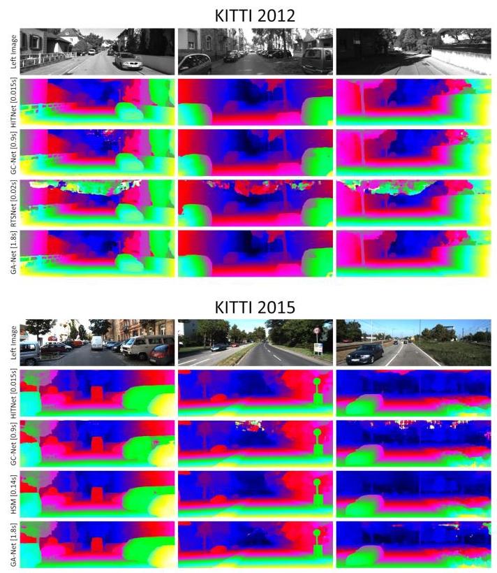
Figure 4: Qualitative Results on KITTI 2012 and 2015. Note how HITNet is able to recover fine structures and crisp edges using a fraction of the computational cost required by other competitors.
图4:KITTI 2012和2015上的定性结果。请注意,HITNet如何能够以其他竞争对手所需计算成本的一小部分恢复精细结构和清晰边缘。
The training set for the real world ETH3D stereo dataset [45] contains just a few stereo pairs, so additional data is needed to avoid overfitting. For the benchmark submission we trained the network on all 394 images from both KITTI datasets, as well as all half and quarter resolution training images from Middlebury dataset V3 [43] and training images from ETH3D dataset. We used the same training parameters as for KITTI submission and stopped training after \({115}\mathrm{k}\) iterations, which was picked using 4 fold cross-validation on ETH3D training set. Note that there is no additional training, pre-training, finetuning.
现实世界ETH3D立体数据集[45]的训练集仅包含少量立体图像对,因此需要额外的数据以避免过拟合。为了提交基准测试结果,我们使用KITTI两个数据集的全部394张图像、Middlebury数据集V3[43]的所有半分辨率和四分之一分辨率训练图像以及ETH3D数据集的训练图像对网络进行训练。我们使用与KITTI提交时相同的训练参数,并在\({115}\mathrm{k}\)次迭代后停止训练,该迭代次数是通过对ETH3D训练集进行4折交叉验证选定的。请注意,没有额外的训练、预训练或微调。
Similarly, the Middlebury dataset [43] contains a limited training set. To avoid overfitting, we pre-trained the model on SceneFlow's FlyingThings TRAIN set with data augmentation, then fine-tuned on the 23 Middlebury14- perfectH training images, while keeping all data augmentations on. Specifically, we used a HITNet Large model with initialization at 6 scales \(\left( {\mathrm{M} = 5}\right)\) , pre-trained it for \({445}\mathrm{k}\) iterations, using batch size of 8 and random crops of \({512} \times {960}\) . We initialize the learning rate to \(4{e}^{-4}\) , then gradually drop it to \(1{e}^{-4},4{e}^{-5}\) and \(1{e}^{-5}\) after \({300}\mathrm{\;K},{400}\mathrm{\;K},{435}\mathrm{\;K}\) iterations respectively. Finally, we fine-tuned the model for \(5\mathrm{\;K}\) iterations at \(1{e}^{-5}\) learning rate. These parameters were selected by using 4-fold cross validation on Middlebury training set.
同样,Middlebury数据集[43]的训练集有限。为避免过拟合,我们在SceneFlow的FlyingThings训练集上进行数据增强后对模型进行预训练,然后在23张Middlebury14 - perfectH训练图像上进行微调,同时保持所有数据增强操作开启。具体而言,我们使用了一个在6个尺度\(\left( {\mathrm{M} = 5}\right)\)上初始化的HITNet大型模型,对其进行\({445}\mathrm{k}\)次迭代的预训练,使用的批量大小为8,随机裁剪尺寸为\({512} \times {960}\)。我们将学习率初始化为\(4{e}^{-4}\),然后分别在\({300}\mathrm{\;K},{400}\mathrm{\;K},{435}\mathrm{\;K}\)次迭代后逐渐将其降至\(1{e}^{-4},4{e}^{-5}\)和\(1{e}^{-5}\)。最后,我们以\(1{e}^{-5}\)的学习率对模型进行\(5\mathrm{\;K}\)次迭代的微调。这些参数是通过对Middlebury训练集进行4折交叉验证选定的。
A.2. Data Augmentation
A.2. 数据增强
The training data available may not be fully representative of the actual test sets for small real world datasets such as KITTI, ETH3D and Middlebury. Indeed, we often observed substantial differences at test time, such as changes in brightness, unexpected reflections and mis-calibrations. In order to improve the network robustness we performed the following augmentations. We first perturb the brightness and contrast of left and right images by using random symmetric and asymmetric multiplicative adjustments. Symmetric adjustments are sampled within \(\left\lbrack {{0.8},{1.2}}\right\rbrack\) interval and asymmetric between \(\left\lbrack {{0.95},{1.05}}\right\rbrack\) . Similar to [55], We then replace random areas of the right image with random crops taken from another portion of the right image: this helps the network to deal with occluded areas and encourages a better "inpainting". The crop size to be replaced is randomly sampled between [50,50] and [180, 250].
对于KITTI、ETH3D和Middlebury等小型现实世界数据集,可用的训练数据可能无法完全代表实际测试集。实际上,我们在测试时经常观察到显著差异,例如亮度变化、意外反射和校准误差。为了提高网络的鲁棒性,我们进行了以下增强操作。我们首先通过随机对称和非对称乘法调整来扰动左右图像的亮度和对比度。对称调整在\(\left\lbrack {{0.8},{1.2}}\right\rbrack\)区间内采样,非对称调整在\(\left\lbrack {{0.95},{1.05}}\right\rbrack\)区间内采样。与文献[55]类似,然后我们用从右图像另一部分随机裁剪的区域替换右图像的随机区域:这有助于网络处理遮挡区域,并促进更好的“图像修复”。要替换的裁剪区域大小在[50,50]和[180, 250]之间随机采样。
Finally, the Middlebury images contains a substantially different color distribution compared to other datasets. To mitigate this we used the approach from [48] that brings color distribution of training images closer to that of Middlebury set and during test time we normalize color distribution between left and right images of a stereopair. Additionally, similar to [55], in order to deal with miscalibrated pairs of this dataset, we augmented the training data with random \(y\) offset between \(\left\lbrack {-2,2}\right\rbrack\) pixels. The random values for \(y\) offset are generated at a low resolution [H/64, W/64], and then bilineraly up-sampled to full resolution \(\left\lbrack {\mathrm{H},\mathrm{W}}\right\rbrack\) of the input image. To simulate different noise levels images with different exposure contain, we add Gaussian random noise with variance sampled between \(\left\lbrack \begin{array}{lll} 0 & {and} & 5 \end{array}\right\rbrack\) intensity levels once for the whole image.
最后,与其他数据集相比,Middlebury图像的颜色分布有很大不同。为了缓解这一问题,我们采用了文献[48]中的方法,使训练图像的颜色分布更接近Middlebury数据集的颜色分布,并且在测试时,我们对立体图像对的左右图像之间的颜色分布进行归一化。此外,与文献[55]类似,为了处理该数据集校准错误的图像对,我们在训练数据中增加了\(y\)随机偏移,偏移量在\(\left\lbrack {-2,2}\right\rbrack\)像素之间。\(y\)偏移的随机值在低分辨率[H/64, W/64]下生成,然后通过双线性插值上采样到输入图像的全分辨率\(\left\lbrack {\mathrm{H},\mathrm{W}}\right\rbrack\)。为了模拟不同曝光的图像所包含的不同噪声水平,我们为整个图像一次性添加方差在\(\left\lbrack \begin{array}{lll} 0 & {and} & 5 \end{array}\right\rbrack\)强度水平之间采样的高斯随机噪声。
B. Additional Evaluations
B. 额外评估
In this section we show additional qualitative results on real-world datasets. In Figure 4 we show comparisons of our method with other approaches. We consider multiple representative competitors such as: GC-Net [24], which uses the full cost volume and 3D convolutions to infer context, RTS-Net [29] that has similar inference time than HIT-Net, and finally GA-Net [61], as one of the best performing methods in terms of accuracy.
在本节中,我们展示了在现实世界数据集上的额外定性结果。在图4中,我们展示了我们的方法与其他方法的比较。我们考虑了多个有代表性的竞争对手,例如:GC - Net[24],它使用完整的代价体和3D卷积来推断上下文;RTS - Net[29],其推理时间与HIT - Net相似;最后是GA - Net[61],它是在准确性方面表现最好的方法之一。
Our method compares very favorably to other approaches such as GC-Net and fast methods like RTSNet and is on par with the state-of-the-art approaches, e.g. GA-Net [61]. Note how our method retrieves fine structures and crisp edges, while only training on the KITTI datasets, which exhibit significant edge fattening artifacts.
我们的方法与其他方法(如GC - Net)以及快速方法(如RTSNet)相比具有显著优势,并且与最先进的方法(例如GA - Net [61])处于同一水平。请注意,我们的方法仅在KITTI数据集上进行训练,就能恢复精细结构和清晰边缘,而KITTI数据集存在明显的边缘模糊伪影。
Similarly, in Figure 7 we show qualitative results on the Middlebury dataset [43]. For each image, we compare HIT-Net with the best performing competitor on the Bad 0.5 metric. Note how our method is able to produce crisp edges, correct occlusions and thin structures in all the considered cases.
同样,在图7中,我们展示了在Middlebury数据集[43]上的定性结果。对于每张图像,我们将HIT - Net与在Bad 0.5指标上表现最佳的竞争对手进行比较。请注意,在所有考虑的情况下,我们的方法都能够产生清晰的边缘、正确处理遮挡并恢复细结构。
B.1. Intermediate Outputs
B.1. 中间输出
We show intermediate outputs from within our network in Fig 6. We observe that with increasing resolution the disparity gets more fine grained and the details from the higher resolution initialization gets merged into the global context that is coming from the lower resolutions. Note that our results on the KITTI 2015 dataset are only trained on the KITTI datasets from scratch without any pre-training on other data sources. This means the network has not been supervised on the top one third of the image as these datasets do only provide ground truth for the bottom two thirds of the image.
我们在图6中展示了网络内部的中间输出。我们观察到,随着分辨率的提高,视差变得更加精细,并且来自高分辨率初始化的细节会融入到来自低分辨率的全局上下文中。请注意,我们在KITTI 2015数据集上的结果是仅在KITTI数据集上从头开始训练得到的,没有在其他数据源上进行任何预训练。这意味着网络没有对图像的前三分之一部分进行监督,因为这些数据集仅为图像的后三分之二部分提供了真实标签。
B.2. Generalization.
B.2. 泛化能力
We finally demonstrate the cross-domain adaptation capabilities of our method. Following the protocol in [49], we trained HITNet on SceneFlow with data augmentations and tested on KITTI 2012 and KITTI 2015 respectively. We also considered multiple competitors as in [49] and report the results in Tab. 5: note how our method shows superior generalization results compared to all the other state-of-the-art approaches. This shows that our method is able to effectively generalize to unseen dataset even without explicit fine-tuning.
最后,我们展示了我们方法的跨领域适应能力。按照文献[49]中的协议,我们在SceneFlow数据集上对HITNet进行了数据增强训练,并分别在KITTI 2012和KITTI 2015数据集上进行了测试。我们还像文献[49]中一样考虑了多个竞争对手,并在表5中报告了结果:请注意,与所有其他最先进的方法相比,我们的方法显示出了更优越的泛化结果。这表明我们的方法即使没有进行显式的微调,也能够有效地泛化到未见过的数据集。
B.3. Ablation Study
B.3. 消融实验
We analyze the importance of our proposed components. The full HITNet is considered as baseline and compared with a version where features are removed. The ablation study is performed on the SceneFlow "finalpass" data and KITTI 2012. See Figure 8 for a qualitative evaluation.
我们分析了我们提出的组件的重要性。将完整的HITNet作为基线,并与去除了某些特征的版本进行比较。消融实验在SceneFlow “finalpass” 数据和KITTI 2012数据集上进行。定性评估结果见图8。
Multi Scale Prediction. The multi-scale feature affects both initialization and propagation stages. In Tab. 6, we report the results for the full model (HITNet) on KITTI 2012, with 5 scales, results for 4 scales and finally we removed the multi-resolution prediction completely. When we evaluated the same settings on the synthetic SceneFlow dataset we did not find a substantial differences between a single scale or multiple ones: clearly the synthetic dataset contains much more textured regions that do not benefit of additional context during propagation, whereas real world scenarios are full of textureless scenes (e.g. walls), where the multi-resolution approach is naturally performing better.
多尺度预测。多尺度特征会影响初始化和传播阶段。在表6中,我们报告了完整模型(HITNet)在KITTI 2012数据集上使用5个尺度的结果、使用4个尺度的结果,最后还报告了完全去除多分辨率预测的结果。当我们在合成的SceneFlow数据集上评估相同的设置时,我们发现单尺度和多尺度之间没有实质性差异:显然,合成数据集包含更多有纹理的区域,这些区域在传播过程中不会从额外的上下文信息中受益,而现实世界场景中充满了无纹理的场景(例如墙壁),在这些场景中,多分辨率方法自然表现更好。
\(4\mathbf{x}4\mathbf{x}4\) Downsampled. Initialization at full disparity resolution provides a compelling starting point to the network, which can focus mostly on refining the prediction. In Tab. 6 we show that using tile resolution for disparity (cost volume is \(4\mathrm{X}\) downsampled in \(\mathrm{H},\mathrm{W}\) and \(\mathrm{D}\) dimensions), the accuracy substantially drops. This demonstrates the importance of our proposed fast high resolution initialization.
\(4\mathbf{x}4\mathbf{x}4\) 下采样。以全视差分辨率进行初始化可为网络提供一个有力的起点,使网络能够主要专注于细化预测。在表6中,我们表明使用分块分辨率进行视差计算(代价体在\(4\mathrm{X}\)和\(\mathrm{D}\)维度上进行\(\mathrm{H},\mathrm{W}\)下采样),准确率会大幅下降。这证明了我们提出的快速高分辨率初始化的重要性。
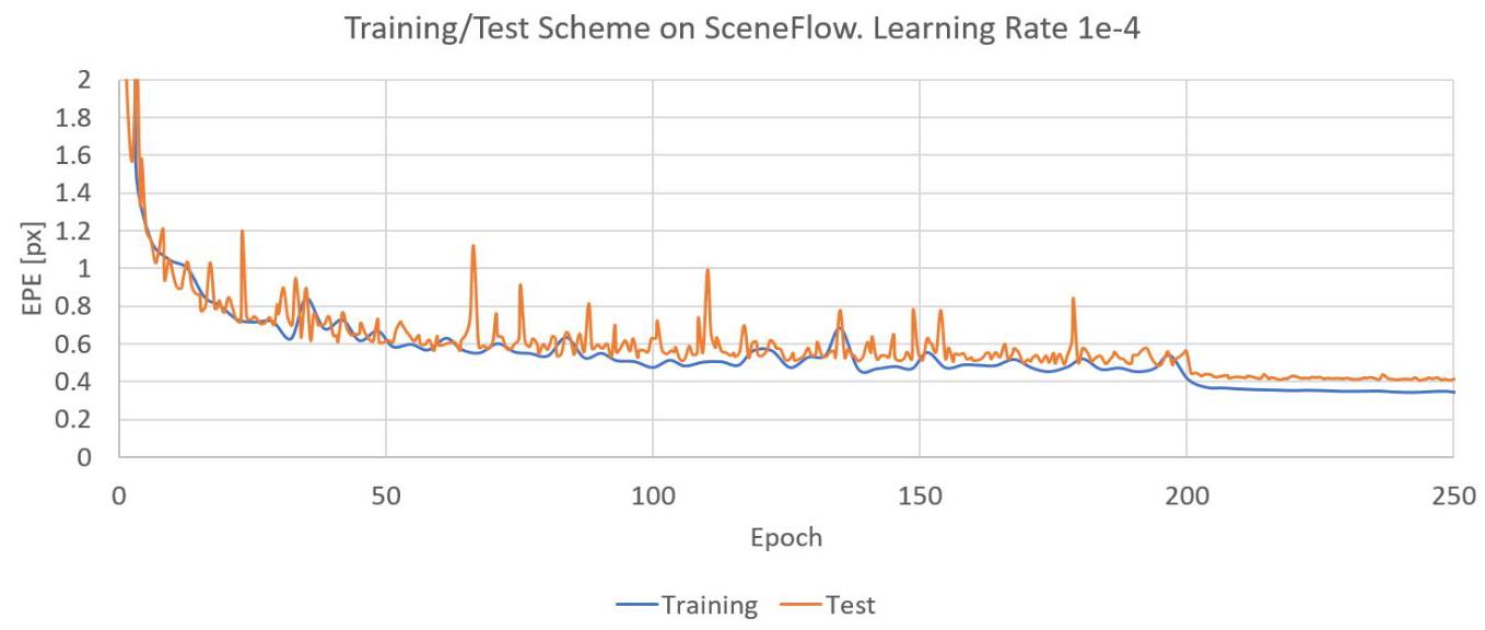
Figure 5: We show the evolution of the training reporting the EPE on training and test set respectively. Note how the scheme reduces the error on both training and test set without showing signs of overfitting.
图5:我们分别报告了训练集和测试集上的端点误差(EPE),展示了训练过程的演变。请注意,该方案在训练集和测试集上都降低了误差,且没有出现过拟合的迹象。
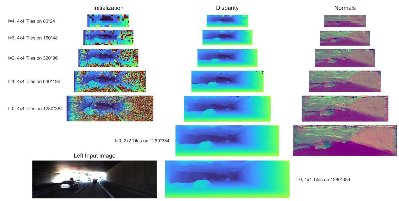
Figure 6: Intermediate results of our network on the left side we show the disparity maps that the matching of the initialization stage provides. On the right hand side we show the final disparity and normals for each resolution. The final two resolutions are \(2\mathrm{x}2\) and \(1\mathrm{x}1\) tiles of the highest resolution feature map, while the initialization is always computed on \(4\mathrm{x}4\) tiles of the feature maps.
图6:我们网络的中间结果。在左侧,我们展示了初始化阶段匹配得到的视差图。在右侧,我们展示了每个分辨率下的最终视差和法线。最后两个分辨率是最高分辨率特征图的\(2\mathrm{x}2\)和\(1\mathrm{x}1\)分块,而初始化始终在特征图的\(4\mathrm{x}4\)分块上进行计算。
\({16} \times {16} \times 8\) Downsampled. Decreasing the resolution of the cost volume for all dimensions similar to [50] degrades accuracy (16X downsampled in \(\mathrm{H}\) and \(\mathrm{W},8\mathrm{X}\) in \(\mathrm{D}\) ). \({16} \times {16} \times 1\) Downsampled. Using larger tiles, while maintaining disparity resolution degrades accuracy even more, as the network is not able to reason about precise disparity at low spatial resolution during initialization.
\({16} \times {16} \times 8\) 下采样。与文献[50]类似,降低代价体所有维度的分辨率会降低准确率(在\(\mathrm{H}\)和\(\mathrm{W},8\mathrm{X}\)维度上进行16倍下采样,在\(\mathrm{D}\)维度上进行下采样)。\({16} \times {16} \times 1\) 下采样。在保持视差分辨率的同时使用更大的分块会进一步降低准确率,因为网络在初始化阶段无法在低空间分辨率下推断出精确的视差。
Slant Prediction. In this experiment, we forced tile hypotheses to always be fronto parallel by setting \({d}_{x}\) and \({d}_{y}\) to 0 and using bilinear interpolation for upsampling. As showed in Tab. 6, removing the slant prediction leads to a substantial drop in precision for both SceneFlow and KITTI 2012. Moreover the network loses its inherent capability of predicting some notion of surface normals that can be useful for many applications such as plane detection.
倾斜预测。在本实验中,我们通过将\({d}_{x}\)和\({d}_{y}\)设为 0,并使用双线性插值进行上采样,强制瓦片假设始终与正面平行。如表 6 所示,去除倾斜预测会导致 SceneFlow 和 KITTI 2012 的精度大幅下降。此外,网络会失去预测表面法线概念的固有能力,而这一能力在许多应用(如平面检测)中非常有用。
| Dataset | HITNet | CRL [40] | iResNet [32] | PSMNet [7] | EdgeStereo [49] |
| KITTI 2012 EPE | 1.06 | 1.38 | 1.27 | 5.54 | 1.96 |
| KITTI 2012 $> {3px}$ | 6.44 | 9.07 | 7.89 | 27.33 | 12.27 |
| KITTI 2015 EPE | 1.36 | 1.35 | 1.21 | 6.44 | 2.06 |
| KITTI 2015 $> {3px}$ | 6.49 | 8.88 | 7.42 | 29.86 | 12.46 |
Table 5: Generalization Experiment. We trained each method on SceneFlow with data augmentation and tested on KITTI 2012 and 2015. Note how our method outperforms the others.
表 5:泛化实验。我们在 SceneFlow 上使用数据增强对每种方法进行训练,并在 KITTI 2012 和 2015 上进行测试。请注意我们的方法是如何优于其他方法的。
| SceneFlow finalpass [38] | KITTI 2012 [15] | ||||||
| Model | EPE | 0.1 px | 1 px | 3 px | EPE | 2 px | 3 px |
| HITNet | 0.529 px | 24.0 % | 5.52 % | 3.00 % | 0.484 px | 2.91 % | 2.00 % |
| 4 Scales | - | - | - | - | 0.507 px | 3.10 % | 2.20 % |
| No Multi-scale | - | - | - | - | 0.747 px | 4.76 % | 3.62 % |
| 4x4x4 Downsampled | 0.561 px | 26.4 % | 5.88 % | 3.15 % | 0.526 px | 3.16 % | 2.19 % |
| 16x16x8 Downsampled | 0.615 px | 27.5 % | 6.36 % | 3.39 % | 0.536 px | 3.35 % | 2.30 % |
| 16x16x1 Downsampled | 0.651 px | 31.9 % | 7.28 % | 3.62 % | 0.554 px | 3.60 % | 2.51 % |
| No Warping | 0.588 px | 31.6 % | 5.88 % | 3.10 % | 0.602 px | 3.72 % | 2.54 % |
| No Slant Prediction | 0.548 px | 25.2 % | 5.74 % | 3.08 % | 0.513 px | 3.23 % | 2.18 % |
| No Tile Features | 0.538 px | 24.7 % | 5.64 % | 3.01 % | 0.488 px | 3.04 % | 2.06 % |
| HITNet L | 0.43 px | 20.7 % | 4.70 % | 2.57 % | 0.490 px | 2.98 % | 2.13 % |
| HITNet XL | 0.36 px | 18.2 % | 4.09 % | 2.21 % | 0.492 px | 3.11 % | 2.20 % |
Table 6: Ablation study of the proposed HITNet on SceneFlow [38] and KITTI 2012 [15] datasets. Lower is better.
表 6:对所提出的 HITNet 在 SceneFlow [38] 和 KITTI 2012 [15] 数据集上的消融研究。数值越低越好。
Tile Features. Here we removed the additional features predicted on each tile during the initialization and propagation steps. This turns out to be a useful component and without it we observe a decrease in accuracy for both datasets.
瓦片特征。在这里,我们去除了在初始化和传播步骤中为每个瓦片预测的额外特征。事实证明,这是一个有用的组件,没有它,我们会发现两个数据集的准确率都会下降。
Warping. The image warps are used to compute the matching cost during the propagation. Removing this step hurts the subpixel precision as demonstrated in Tab. 6.
翘曲。图像翘曲用于在传播过程中计算匹配成本。如表 6 所示,去除这一步骤会损害亚像素精度。
Model Size. Finally, we tested if an increase in the model size is beneficial or not. In particular we double the channels in the feature extractor, and use 32 channels and 6 residual blocks for the last 3 propagation steps, this resorts to a run-time increase to \({54}\mathrm{\;{ms}}\) . As expected this has an improvement on SceneFlow as reported in Tab. 6, HITNet Large; however for the small KITTI datasets this did not improve performance due to over-fitting. Further increasing model size by using 64 channels for the last 3 propagation steps improved SceneFlow results, increased runtime to \({114}\mathrm{\;{ms}}\) , and increased over-fitting on a smaller dataset. We don't see a reason to explore larger model sizes on a synthetic dataset as it will add to over-fitting on smaller real datasets that are publicly available. The metrics on "clean-pass" for XL version are: 0.31 epe, 15.6 bad 0.1, 3.67 bad 1.0,1.99bad 3.0.
模型大小。最后,我们测试了增加模型大小是否有益。具体来说,我们将特征提取器中的通道数增加一倍,并在最后 3 个传播步骤中使用 32 个通道和 6 个残差块,这导致运行时间增加到\({54}\mathrm{\;{ms}}\)。如表 6 中 HITNet Large 所示,正如预期的那样,这对 SceneFlow 有改进;然而,对于较小的 KITTI 数据集,由于过拟合,性能并没有得到改善。通过在最后 3 个传播步骤中使用 64 个通道进一步增加模型大小,改善了 SceneFlow 的结果,运行时间增加到\({114}\mathrm{\;{ms}}\),并且在较小的数据集上增加了过拟合。我们认为没有必要在合成数据集上探索更大的模型大小,因为这会增加在公开可用的较小真实数据集上的过拟合。XL 版本在“干净通道”上的指标为:0.31 端点误差(epe),15.6% 误差大于 0.1,3.67% 误差大于 1.0,1.99% 误差大于 3.0。
C. Model Architecture Details
C. 模型架构细节
By default, the HITNet architecture is implemented with a 5-scale feature extractor with16,16,24,24,32channels at corresponding resolutions. During Initialization step the first convolution over \(4 \times 4\) tiles outputs 16 channels, followed by 2-layer MLP with 32 and 16 channels and ReLU non-linearities. Tile descriptor has 13 channels by default, residual blocks use 32 channels, unless mentioned otherwise. Each intermediate propagation steps use 2 residual blocks without dilations. At each spatial resolutions, the propagation module uses feature maps from appropriate scale: full-resolution feature maps for \(4 \times 4\) tiles, \(2\mathrm{X}\) downsampled for coarser tiles that have size \(8 \times 8\) in full resolution, but sample \(4 \times 4\) pixels in coarser feature map, etc till \({16}\mathrm{X}\) downsampled and \({64} \times {64}\) tiles in original resolution. The last 3 levels of propagation start at \(4 \times 4\) tiles and progressively in-paint and refine strong correct disparity at the edges over larger regions. To achieve that, they operate on coarse feature maps: the \(4 \times 4\) tiles use \(4\mathrm{X}\) downsampled features for warping, the \(2 \times 2\) tiles use \(2\mathrm{X}\) downsampled features for warping, the \(1 \times 1\) tiles use full-resolution features for warping.
默认情况下,HITNet 架构使用 5 尺度特征提取器实现,在相应分辨率下具有 16、16、24、24、32 个通道。在初始化步骤中,对\(4 \times 4\)个瓦片的第一次卷积输出 16 个通道,随后是具有 32 和 16 个通道以及 ReLU 非线性激活函数的两层多层感知机(MLP)。默认情况下,瓦片描述符有 13 个通道,残差块使用 32 个通道,除非另有说明。每个中间传播步骤使用 2 个无膨胀的残差块。在每个空间分辨率下,传播模块使用来自适当尺度的特征图:\(4 \times 4\)个瓦片使用全分辨率特征图,对于在全分辨率下大小为\(8 \times 8\)但在较粗特征图中采样\(4 \times 4\)个像素的较粗瓦片,使用\(2\mathrm{X}\)下采样的特征图,以此类推,直到\({16}\mathrm{X}\)下采样和原始分辨率下的\({64} \times {64}\)个瓦片。最后 3 层传播从\(4 \times 4\)个瓦片开始,逐步在更大区域的边缘内插并细化强正确视差。为了实现这一点,它们在粗特征图上操作:\(4 \times 4\)个瓦片使用\(4\mathrm{X}\)下采样的特征进行翘曲,\(2 \times 2\)个瓦片使用\(2\mathrm{X}\)下采样的特征进行翘曲,\(1 \times 1\)个瓦片使用全分辨率特征进行翘曲。
In HITNet model used in KITTI and ETH3d experiments last 3 propagation steps use4,4,2residual blocks with32,32,16channels and \(1,3,1,1;1,3,1,1;1,1\) dilations.
在 KITTI 和 ETH3d 实验中使用的 HITNet 模型,最后 3 个传播步骤使用具有 32、32、16 个通道和\(1,3,1,1;1,3,1,1;1,1\)膨胀率的 4、4、2 个残差块。
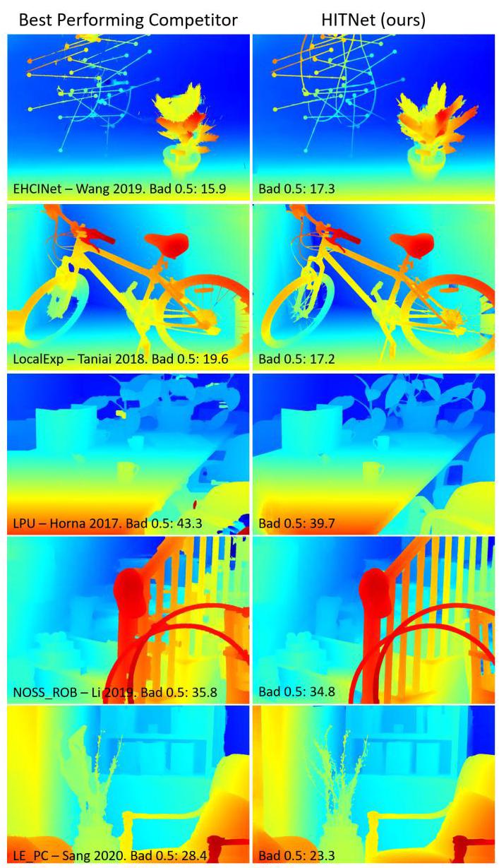
Figure 7: Qualitative comparisons on Middlebury dataset. For each image we compare our method with the best performing competitor following the Bad 0.5 metric. Note how our method is able to produce crisp edges, correct occlusions and thin structures in all the considered cases.
图 7:在 Middlebury 数据集上的定性比较。对于每张图像,我们将我们的方法与根据 Bad 0.5 指标表现最佳的竞争对手进行比较。请注意,在所有考虑的情况下,我们的方法都能够产生清晰的边缘、正确处理遮挡和细化薄结构。
HITNet model used in Sceneflow experiments uses 16,16,24,24,32channels for feature extractor. A single initialization at \(4 \times 4\) tiles. Last 3 propagation steps use6,6,6residual blocks with32,32,16channels and 1,2,4,8,1,1dilations.
场景流(Sceneflow)实验中使用的HITNet模型在特征提取器中使用16、16、24、24、32个通道。在\(4 \times 4\)图块处进行单次初始化。最后3个传播步骤使用6、6、6个残差块(residual blocks),通道数分别为32、32、16,膨胀率(dilations)分别为1、2、4、8、1、1。
HITNetL model used in Sceneflow experiments uses 32,40,48,56,64channels for feature extractor. A single initialization at \(4 \times 4\) tiles. Last 3 propagation steps use6,6,6residual blocks with32,32,32channels and 1,2,4,8,1,1dilations.
场景流(Sceneflow)实验中使用的HITNetL模型在特征提取器中使用32、40、48、56、64个通道。在\(4 \times 4\)图块处进行单次初始化。最后3个传播步骤使用6、6、6个残差块(residual blocks),通道数均为32,膨胀率(dilations)分别为1、2、4、8、1、1。
HITNetXL model used in Sceneflow experiments uses 32,40,48,56,64channels for feature extractor. A single initialization at \(4 \times 4\) tiles. Last 3 propagation steps use6,6,6residual blocks with64,64,64channels and 1,2,4,8,1,1dilations.
场景流(Sceneflow)实验中使用的HITNetXL模型在特征提取器中使用32、40、48、56、64个通道。在\(4 \times 4\)图块处进行单次初始化。最后3个传播步骤使用6、6、6个残差块(residual blocks),通道数均为64,膨胀率(dilations)分别为1、2、4、8、1、1。
HITNet model used in Middlebury experiments uses 32,40,48,56,64channels for feature extractor. Last 3 propagation steps use6,6,6residual blocks with32,32,32 channels and1,2,4,8,1,1dilations.
米德尔伯里(Middlebury)实验中使用的HITNet模型在特征提取器中使用32、40、48、56、64个通道。最后3个传播步骤使用6、6、6个残差块(residual blocks),通道数均为32,膨胀率(dilations)分别为1、2、4、8、1、1。
The models used for submission for benchmarks and scripts to run them are available at https://github.com/google-research/google-research/tree/master/hitnet
用于基准测试提交的模型以及运行这些模型的脚本可在https://github.com/google - research/google - research/tree/master/hitnet获取。
Fig 9 provides more details for the initialization module described in the main paper. Similarly Fig 10 and Fig 11 show how resblocks are integrated into propagation logic. Finally, Fig 12 depicts differences between propagation steps when a single hypothesis or multiple hypotheses are used.
图9为主论文中描述的初始化模块提供了更多细节。类似地,图10和图11展示了残差块(resblocks)如何集成到传播逻辑中。最后,图12描绘了使用单一假设或多个假设时传播步骤之间的差异。
D. Runing Time Details
D. 运行时间详情
The HITNet architecture used for ETH3d and KITTI experiments runs at \({19}\mathrm{\;{ms}}\) per frame on a Titan V GPU for 0.5Mpixel (KITTI resolution) input images. The majority of the time is spent during the last 3 propagation steps \({7.5}\mathrm{\;{ms}}\) ) that operate on higher resolutions. The multi-scale propagation steps use down-sampled data and contribute less than \(5\mathrm{\;{ms}}\) . Efficient implementation of initialization using a single fused \(\mathrm{{Op}}\) generates initial disparity estimates across all resolutions in \({0.25}\mathrm{\;{ms}}\) , with feature extractor contributing \(6\mathrm{\;{ms}}\) . For Middlebury experiments the model has a run-time of approximately \({107.5}\mathrm{\;{ms}}\) per Mpix of input resolution using custom CUDA operations for initialization and warping, when maximum disparity is 160 and the run-time scales linearly with resolution. The run-time has a small increase with disparity range, and is about \({109}\mathrm{\;{ms}}\) per Mpix for a maximum disparity of 1024. Without custom CUDA operations the run-time is increased by a factor of 3 , as a single warping operation contains more than a hundred simple operations over large tensors, and while it's trivial to fuse them together, not doing so results in most of the time spent on global memory access. When tested on an 18-core Xeon 6154 CPU, the default tensorflow runtime runs 3.3s per Mpix, which would translate to about \({60s}\) for a single threaded runtime, which compares favourably to other CPU methods. The CPU tensorflow runtime does make use of SIMD instruction set, which other methods may not utilize.
用于ETH3d和基蒂(KITTI)实验的HITNet架构,对于0.5M像素(基蒂(KITTI)分辨率)的输入图像,在Titan V GPU上每帧运行时间为\({19}\mathrm{\;{ms}}\)。大部分时间花费在最后3个在较高分辨率上操作的传播步骤(\({7.5}\mathrm{\;{ms}}\))。多尺度传播步骤使用下采样数据,其耗时不到\(5\mathrm{\;{ms}}\)。使用单个融合的\(\mathrm{{Op}}\)进行高效初始化,可在\({0.25}\mathrm{\;{ms}}\)内生成所有分辨率的初始视差估计,特征提取器耗时为\(6\mathrm{\;{ms}}\)。对于米德尔伯里(Middlebury)实验,当最大视差为160时,使用自定义CUDA操作进行初始化和扭曲,该模型每兆像素输入分辨率的运行时间约为\({107.5}\mathrm{\;{ms}}\),且运行时间与分辨率呈线性关系。视差范围增大时,运行时间略有增加,最大视差为1024时,每兆像素的运行时间约为\({109}\mathrm{\;{ms}}\)。如果不使用自定义CUDA操作,运行时间会增加3倍,因为单个扭曲操作包含对大张量的一百多个简单操作,虽然将它们融合在一起很简单,但不这样做会导致大部分时间花费在全局内存访问上。在18核至强(Xeon)6154 CPU上测试时,默认的TensorFlow运行时每兆像素运行时间为3.3秒,单线程运行时约为\({60s}\),这与其他CPU方法相比具有优势。CPU的TensorFlow运行时确实利用了单指令多数据(SIMD)指令集,而其他方法可能未使用。
E. Number of Parameters
E. 参数数量
An important aspect of efficient neural network architectures is the number of parameters they have. This will influence the amount of compute required and the amount of memory needed to store them. Moreover, being able to achieve good performance with fewer numbers of parameters makes the network less susceptible to over-fitting. In Tab. 7 we show that our network is able to achieve better results than other approaches with a significantly lower number of parameters and compute.
高效神经网络架构的一个重要方面是其参数数量。这将影响所需的计算量和存储所需的内存量。此外,能够以较少的参数数量实现良好的性能,可使网络更不易过拟合。在表7中,我们展示了我们的网络能够以显著更少的参数数量和计算量取得比其他方法更好的结果。
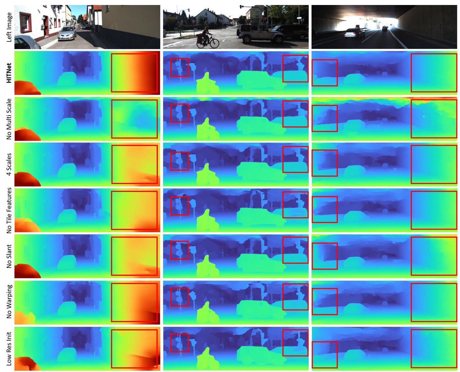
Figure 8: Ablation study, qualitative evaluation. Note how our HITNet model relies on all proposed design choices in order to achieve the best results on fine details, edges and occluded regions.
图8:消融研究,定性评估。请注意,我们的HITNet模型如何依赖所有提出的设计选择,以便在精细细节、边缘和遮挡区域上取得最佳结果。
| Model | Param | GMac | EPE | 1 Pixel Threshold Error Rates |
| GC-Net [24] | 2.9M [61] | 8789 [6] | 1.80 [61] | 15.6 [61] |
| PSMNet [7] | 3.5M [61] | 2594 [6] | 1.09 [61] | 12.1 [61] |
| GANet [61] | 2.3M [61] | - | 0.84 [61] | 9.9 [61] |
| StereoDRNet [6] | - | 1410 [6] | 0.98 [6] | - |
| LEAStereo [8] | 1.81M [8] | 782 [8] | 0.78 [8] | 7.82 [8] |
| HITNet Single-scale | 0.45M | 52 (92) | 0.53 | 5.52 |
| HITNet Multi-scale | 0.66M | 36 (61) | - | - |
| HITNetL | 0.97M | 146 (235) | 0.43 | 4.56 |
| HITNet Middlebury | 1.62M | 187; 450 for 1.57Mpix input | - | - |
| HITNetXL | 2.07M | 396 (735) | 0.36 | 4.09 |
Table 7: Comparisons of number of parameters and GMacs (Giga Multiply-accumulate operations) with other methods on Scene Flow "finalpass" dataset (960 × 540 inputs). The numbers were partially adopted from the papers cited in the table. The lower the better. The multi-scale version of HITNet is used for ETH3d and KITTI submissions, GMac is provided for \({1280} \times {384}\) inputs. The GMac number in parenthesis is for predicting both disparity maps, sharing the feature extractor.
表7:在场景流(Scene Flow)“最终通道(finalpass)”数据集(960×540输入)上与其他方法在参数数量和千兆乘累加运算(Giga Multiply-accumulate operations,GMacs)方面的比较。表中的部分数据取自表中引用论文。数值越低越好。HITNet的多尺度版本用于ETH3d和KITTI提交,GMac是针对\({1280} \times {384}\)输入给出的。括号中的GMac数值是用于预测两个视差图(共享特征提取器)的。
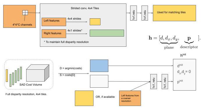
Figure 9: Initialization: The features extracted by the feature extractor are matched and inital tile features are computed. The number of feature channels \(C\) depends on feature extractor architecture and the current level (see Sec. C)
图9:初始化:对特征提取器提取的特征进行匹配,并计算初始图块特征。特征通道数\(C\)取决于特征提取器的架构和当前层级(见C节)
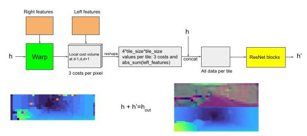
Figure 10: Propagation, for the single hypothesis case.
图10:单假设情况下的传播。
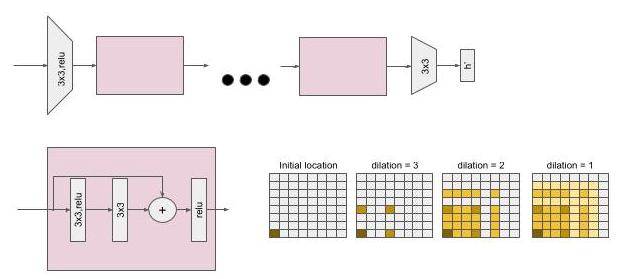
Figure 11: ResNet blocks. First 3x3 convolution generates a local state for the tile, which is incrementally updated by each block. The final state generates tile updates. Each block may use dilated convolutions to increase the speed of diffusion.
图11:残差网络(ResNet)模块。第一个3x3卷积为图块生成一个局部状态,该状态由每个模块逐步更新。最终状态生成图块更新。每个模块可以使用空洞卷积来提高扩散速度。
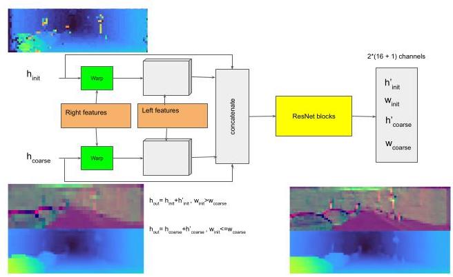
Figure 12: Propagation with multiple hypotheses.
图12:多假设传播。
Having less parameters also increases the generalization capabilities of the proposed method: indeed less learnable weights implies that the network is less prone to overfitting - our approach is able to outperform multiple state-of-the-art baselines when trained on synthetic data and tested in real-world scenarios.
减少参数数量还能增强所提出方法的泛化能力:实际上,可学习的权重越少意味着网络越不容易过拟合——当在合成数据上进行训练并在现实场景中进行测试时,我们的方法能够超越多个最先进的基线方法。

 浙公网安备 33010602011771号