Tensorflow实现LeNet-5、Saver保存与读取

posted @ 2019-03-31 22:53 nxf_rabbit75 阅读(1382) 评论(0) 编辑收藏举报

分类: TensorFlow

undefined

一、 LeNet-5

LeNet-5是一种用于手写体字符识别的非常高效的卷积神经网络。
卷积神经网络能够很好的利用图像的结构信息。
卷积层的参数较少，这也是由卷积层的主要特性即局部连接和共享权重所决定。

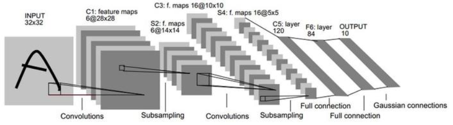
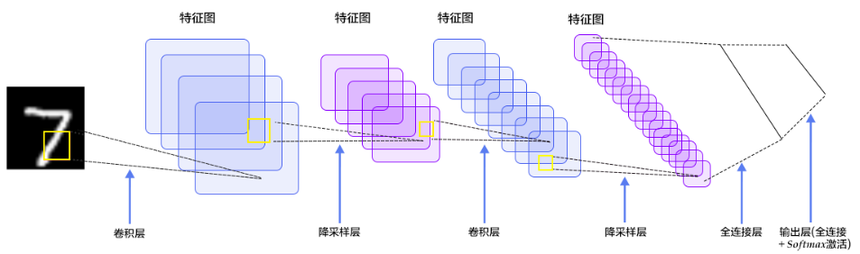
　　LeNet-5共有7层，不包含输入，每层都包含可训练参数；每个层有多个Feature Map，每个FeatureMap通过一种卷积滤波器提取输入的一种特征，然后每个FeatureMap有多个神经元。

数据集：mnist

train-images-idx3-ubyte 训练数据图像 (60,000)
train-labels-idx1-ubyte 训练数据label
t10k-images-idx3-ubyte 测试数据图像 (10,000)
t10k-labels-idx1-ubyte 测试数据label

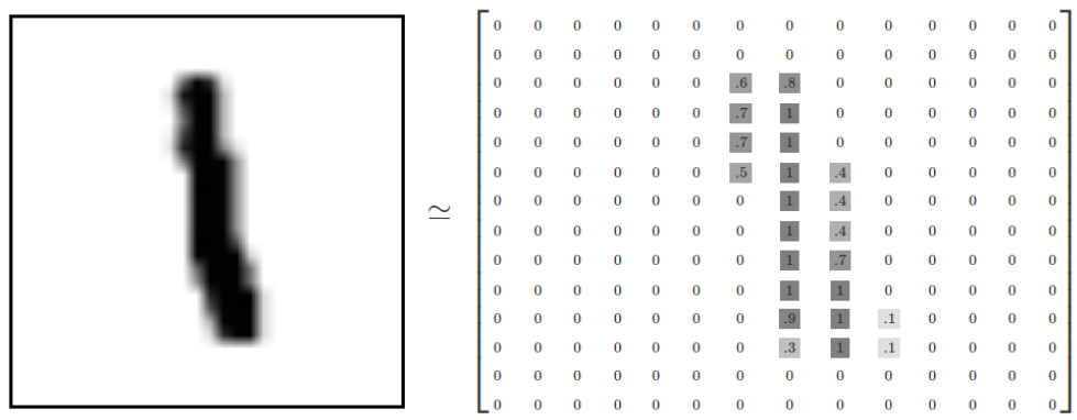
每张图像是28*28像素：

　　我们的任务是使用上面数据训练一个可以准确识别手写数字的神经网络模型，并使用Tensorflow对训练过程各个参数的变化进行可视化。

1. 准备数据集、定义超参数等准备工作

（1）导入需要使用的包

import tensorflow as tf
from tensorflow.examples.tutorials.mnist import input_data
 
# gpu设置
import os
os.environ["CUDA_VISIBLE_DEVICES"] = "0"
config = tf.ConfigProto(allow_soft_placement = True)
gpu_options = tf.GPUOptions(per_process_gpu_memory_fraction = 0.33)
config.gpu_options.allow_growth = True<br><br>mnist=input_data.read_data_sets('MNIST_data',one_hot=True)

上述代码的意思是使用GPU设备0，最多给GPU分配总共内存的百分之33，并且允许GPU按需申请内存。也就是说，假设一个程序使用一块GPU内存百分之10就够了，如果我们没有指定allow_growth=True，那么程序会直接占用GPU内存的百分之33，因为这个是我们给它分配的。如果我们连0.33，也就是GPU内存的百分之33都没有指定，那么程序会直接占用整个GPU设备0。虽然占用这么多没有用，但是我就占着，属于“占着茅坑不拉屎”。所以，为了充分利用资源，特别是一帮人使用一个服务器的时候，指定下这些参数就很有必要了。

2. 数据处理

（1）创建输入数据的占位符，分别创建特征数据xs，标签数据ys

　　在tf.placeholder()函数中传入了3个参数，第一个是定义数据类型为float32；第二个是数据的大小，特征数据是大小784的向量，标签数据是大小为10的向量，None表示不确定死大小，到时候可以传入任何数量的样本；第3个参数是这个占位符的名称。

sess=tf.Session()
 
# 创建输入数据的占位符，分别创建特征数据xs，标签数据ys
with tf.name_scope('input'):
    xs=tf.placeholder(tf.float32,[None,784])
    ys=tf.placeholder(tf.float32,[None,10])
 
keep_prob=tf.placeholder(tf.float32)

　　mnist下载好的数据集就是很多个1*784的向量，就是已经对28*28的图片进行了向量化处理。

（2）使用tf.summary.image保存图像信息

　　特征数据其实就是图像的像素数据拉升成一个1*784的向量，现在如果想在tensorboard上还原出输入的特征数据对应的图片，就需要将拉升的向量转变成28 * 28 * 1的原始像素了，于是可以用tf.reshape()直接重新调整特征数据的维度：

　　将输入的数据转换成[28 * 28 * 1]的shape，存储成另一个tensor，命名为image_shaped_input。为了能使图片在tensorbord上展示出来，使用tf.summary.image将图片数据汇总给tensorbord。tf.summary.image（）中传入的第一个参数是命名，第二个是图片数据，第三个是最多展示的张数，此处为10张。

# 保存图像信息
with tf.name_scope('input_reshape'):
    image_shaped_input = tf.reshape(x, [-1, 28, 28, 1])
    tf.summary.image('input', image_shaped_input, 10)

3. 初始化参数并保存参数信息到summary

（1）初始化参数w和b

　　在构建神经网络模型中，每一层中都需要去初始化参数w,b,为了使代码简介美观，最好将初始化参数的过程封装成方法function。创建初始化权重w的方法，生成大小等于传入的shape参数，标准差为0.1，遵循正态分布的随机数，并且将它转换成tensorflow中的variable返回。

def weight_variable(shape): 
    initial=tf.truncated_normal(shape,stddev=0.1) #tf.truncted_normal产生随机变量来进行初始化,类似normal  
    return tf.Variable(initial)

　　创建初始换偏执项b的方法，生成大小为传入参数shape的常数0.1，并将其转换成tensorflow的variable并返回。

def bias_variable(shape): 
    initial=tf.constant(0.1,shape=shape) 
    return tf.Variable(initial)

（2）记录训练过程参数变化

　　我们知道，在训练的过程在参数是不断地在改变和优化的，我们往往想知道每次迭代后参数都做了哪些变化，可以将参数的信息展现在tenorbord上，因此我们专门写一个方法来收录每次的参数信息。

# 绘制参数变化
def variable_summaries(var):
    with tf.name_scope('summaries'):
        # 计算参数的均值，并使用tf.summary.scaler记录
        mean = tf.reduce_mean(var)
        tf.summary.scalar('mean', mean)
 
        # 计算参数的标准差
        with tf.name_scope('stddev'):
            stddev = tf.sqrt(tf.reduce_mean(tf.square(var - mean)))
        # 使用tf.summary.scaler记录记录下标准差，最大值，最小值
        tf.summary.scalar('stddev', stddev)
        tf.summary.scalar('max', tf.reduce_max(var))
        tf.summary.scalar('min', tf.reduce_min(var))
        # 用直方图记录参数的分布
        tf.summary.histogram('histogram', var)

4. 搭建神经网络层　

（1）定义卷积层、max_pool层

　　定义卷积，tf.nn.conv2d函数是tensoflow里面的二维的卷积函数，x是图片的所有参数，W是此卷积层的权重，然后定义步长strides=[1,1,1,1]值，strides[0]和strides[3]的两个1是默认值，中间两个1代表padding时在x方向运动一步，y方向运动一步，padding采用的方式是SAME。

1 2	`def` `conv2d(x,W):` `return` `tf.nn.conv2d(x,W,strides=[1,1,1,1],padding='SAME')`

　　接着定义池化pooling，为了得到更多的图片信息，padding时我们选的是一次一步，也就是strides[1]=strides[2]=1，这样得到的图片尺寸没有变化，而我们希望压缩一下图片也就是参数能少一些从而减小系统的复杂度，因此我们采用pooling来稀疏化参数，也就是卷积神经网络中所谓的下采样层。pooling 有两种，一种是最大值池化，一种是平均值池化，本例采用的是最大值池化tf.max_pool()。池化的核函数大小为2x2，因此ksize=[1,2,2,1]，步长为2，因此strides=[1,2,2,1]

1 2	`def` `max_pool_2x2(x):` `return` `tf.nn.max_pool(x,ksize=[1,2,2,1],strides=[1,2,2,1],padding='SAME')`

（2）建立卷积层conv1，conv2、建立全连接层fc1，fc2

建立卷积层conv1,conv2

# 建立卷积层conv1,conv2
with tf.name_scope('conv1'):
    W_conv1=weight_variable([5,5,1,32])#patch/kernel 5*5,in size 1是image的厚度,out size 32
    b_conv1=bias_variable([32]) #一个kernel一个bias
    h_conv1=tf.nn.relu(conv2d(x_image,W_conv1)+b_conv1)#output size 28*28*32
 
with tf.name_scope('max_pool1'):    
    h_pool1=max_pool_2x2(h_conv1) #output size 14*14*32  
 
with tf.name_scope('conv2'):
    W_conv2=weight_variable([5,5,32,64])#kernel 5*5,in size 32,out size 64
    b_conv2=bias_variable([64])#output size 14*14*64
    h_conv2=tf.nn.relu(conv2d(h_pool1,W_conv2)+b_conv2)#output size 7*7*64
 
with tf.name_scope('max_pool2'):
    h_pool2=max_pool_2x2(h_conv2)

建立全连接层fc1，fc2

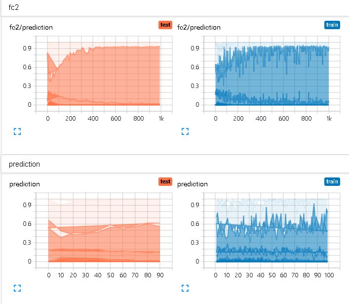
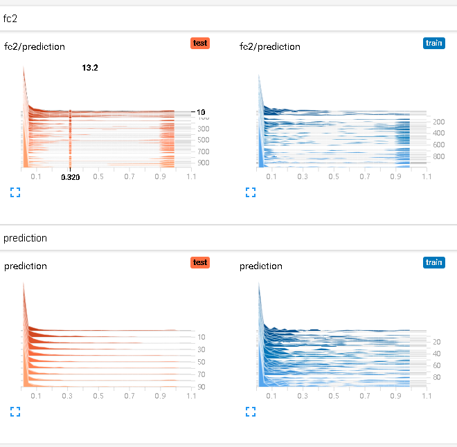
#建立全连接层fc1,fc2
#[n_samples,7,7,64]->>[n_samples,7*7*64]
with tf.name_scope('fc1'):
    h_pool2_flat=tf.reshape(h_pool2,[-1,7*7*64]) 
    W_fc1=weight_variable([7*7*64,1024]) 
    b_fc1=bias_variable([1024])
    h_fc1=tf.nn.relu(tf.matmul(h_pool2_flat,W_fc1)+b_fc1)
    h_fc1_drop=tf.nn.dropout(h_fc1,keep_prob)
    tf.summary.scalar('dropout_keep_probability',keep_prob)
 
with tf.name_scope('fc2'):
    W_fc2=weight_variable([1024,10]) 
    b_fc2=bias_variable([10])
    prediction=tf.nn.softmax(tf.matmul(h_fc1_drop,W_fc2)+b_fc2) #最终的结果
    tf.summary.histogram('prediction',prediction)

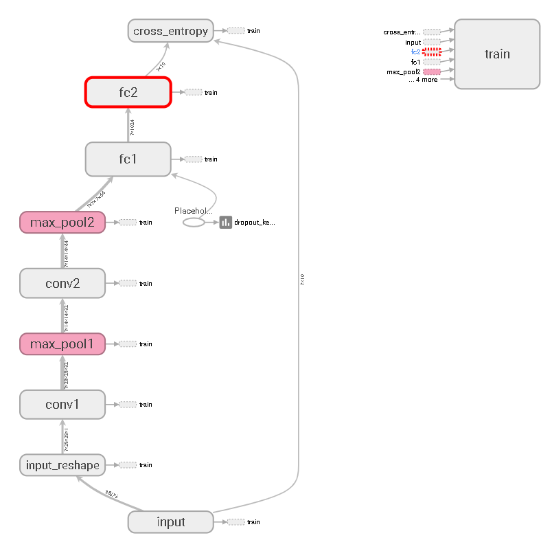
模型可视化：

预测值分布：

预测值直方图：

5. 损失函数与优化

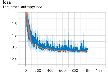
#交叉熵
with tf.name_scope('cross_entropy'):
    cross_entropy=tf.reduce_mean(-tf.reduce_sum(ys*tf.log(prediction),reduction_indices=[1]))
    tf.summary.scalar('loss',cross_entropy)
 
#优化器
with tf.name_scope('train'):
    train_step=tf.train.AdamOptimizer(1e-4).minimize(cross_entropy)

损失值变化：

6. 训练

#所有变量初始化
# summaries合并
merged = tf.summary.merge_all()
 
# 写到指定的磁盘路径中
train_writer = tf.summary.FileWriter('E:/nxf_anaconda_base_jupyter_ht/LeNet/train',sess.graph)
test_writer = tf.summary.FileWriter('E:/nxf_anaconda_base_jupyter_ht/LeNet/test',sess.graph)
 
sess.run(tf.global_variables_initializer())
 
# 计算准确率
with tf.name_scope('accuracy'):
    with tf.name_scope('correct_prediction'):
        # 分别将预测和真实的标签中取出最大值的索引,相同则返回1(true),不同则返回0(false)
        correct_prediction = tf.equal(tf.argmax(prediction, 1), tf.argmax(ys, 1))
    with tf.name_scope('accuracy'):
        # 求均值即为准确率
        accuracy = tf.reduce_mean(tf.cast(correct_prediction, tf.float32))
          
tf.summary.scalar('accuracy', accuracy)

7. 所有变量初始化、送入数据集

　　feed_dict用于获取数据，如果是train==true，也就是进行训练的时候，就从mnist.train中获取一个batch大小为100样本，并且设置dropout值为0.9。如果是不是train==false,则获取minist.test的测试数据，并且设置dropout为1，即保留所有神经元开启。

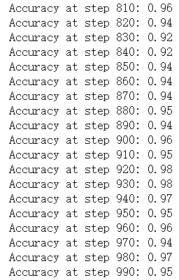
　　同时，每隔10步，进行一次测试，并打印一次测试数据集的准确率，然后将测试数据集的各种summary信息写进日志中。其余的时候，都是在进行训练，将训练集的summary信息并写到日志中。

def feed_dict(train):
    """Make a TensorFlow feed_dict: maps data onto Tensor placeholders."""
    if train:
        x, y = mnist.train.next_batch(10)
        k = 0.9 #dropout
    else:
        x, y = mnist.test.images[100:200], mnist.test.labels[100:200]
        k = 1.0
    return {xs: x, ys: y, keep_prob: k}
  
for i in range(1000):
    if i % 10 == 0:  #记录测试集的summary与accuracy
        summary, acc = sess.run([merged, accuracy], feed_dict=feed_dict(False))
        test_writer.add_summary(summary, i)
        print('Accuracy at step %s: %s' % (i, acc))
    else:  # 记录训练集的summary
        summary, _ = sess.run([merged, train_step], feed_dict=feed_dict(True))
        train_writer.add_summary(summary, i)
         
train_writer.close()
test_writer.close()

二、saver的save和restore

TensorFlow提供了一个非常方便的api，tf.train.Saver()用来保存和还原一个机器学习模型。

程序会生成并保存四个文件:

checkpoint ：文本文件，记录了模型文件的路径信息列表
save_net.ckpt.data-00000-of-00001：网络权重信息
save_net.ckpt.index：.data和.index这两个文件是二进制文件，保存了模型中的变量参数（权重）信息
save_net.ckpt.meta：二进制文件，保存了模型的计算图结构信息（模型的网络结构）protobuf

建立模型

import tensorflow as tf
import numpy as np
 
## Save to file
# remember to define the same dtype and shape when restore
W = tf.Variable([[1,2,3],[3,4,5]], dtype=tf.float32, name='weights')
b = tf.Variable([[1,2,3]], dtype=tf.float32, name='biases')
 
# init= tf.initialize_all_variables() # tf 马上就要废弃这种写法
# 替换成下面的写法:
init = tf.global_variables_initializer()　

变量的保存

saver = tf.train.Saver()
 
with tf.Session() as sess:
    sess.run(init)
    save_path = saver.save(sess, "nxf_net/save_net.ckpt")
    print("Save to path: ", save_path)
 
"""    
Save to path:  nxf_net/save_net.ckpt
"""

变量的重载

# restore variables
# reduce the same shape and same type for your variables
# 先建立W,b的容器
W = tf.Variable(np.arange(6).reshape((2, 3)), dtype=tf.float32, name="weights")
b = tf.Variable(np.arange(3).reshape((1, 3)), dtype=tf.float32, name="biases")
 
# 这里不需要初始化步骤 init= tf.initialize_all_variables()
 
saver = tf.train.Saver()
with tf.Session() as sess:
    # 提取变量
    saver.restore(sess, "my_net/save_net.ckpt")
    print("weights:", sess.run(W))
    print("biases:", sess.run(b))
 
"""
weights: [[ 1.  2.  3.]
          [ 3.  4.  5.]]
biases: [[ 1.  2.  3.]]
"""