Tensorflow 搭建神经网络及tensorboard可视化

posted @ 2019-03-30 11:54 nxf_rabbit75 阅读(684) 评论(0) 编辑收藏举报

分类: TensorFlow

undefined

1. session对话控制

matrix1 = tf.constant([[3,3]])
matrix2 = tf.constant([[2],[2]])
product = tf.matmul(matrix1,matrix2) #类似于numpy的np.dot(m1,m2)

方法1：

sess = tf.Session()
result = sess.run(product)
print(result) # [[12]]
sess.close()

方法2：

with tf.Session() as sess:#不需要手动关闭sess
    result2 = sess.run(product)
    print(result2) # [[12]]

2. Variable变量

state = tf.Variable(0,name='counter')
 
#定义常量 one
one = tf.constant(1)
 
#定义加法步骤（注:此步并没有直接计算）
new_value = tf.add(state,one)
 
#将 State 更新成 new_value
update = tf.assign(state,new_value)
 
# 如果定义 Variable, 就一定要 initialize
# init = tf.initialize_all_variables() # tf 马上就要废弃这种写法
init = tf.global_variables_initializer()  # 替换成这样就好
 
with tf.Session() as sess:
    sess.run(init)
    for _ in range(3):
        sess.run(update)
        print(sess.run(state))
 
>>>1
2
3

3. placeholder

　　Tensorflow 如果想要从外部传入data, 那就需要用到 tf.placeholder(), 然后以这种形式传输数据 sess.run(***, feed_dict={input: **}).

接下来, 传值的工作交给了 sess.run() , 需要传入的值放在了feed_dict={} 并一一对应每一个 input. placeholder 与 feed_dict={} 是绑定在一起出现的。

input1 = tf.placeholder(tf.float32) #大部分只能处理float32
input2 = tf.placeholder(tf.float32) #两行两列[2,2]
 
output = tf.multiply(input1,input2)
 
with tf.Session() as sess:
    print(sess.run(output,feed_dict={input1:[2.],input2:[1.]}))
 
>>>[2.]

4. 添加层def add_layer()

import tensorflow as tf
 
def add_layer(inputs,in_size,out_size,activation_function=None):
    with tf.name_scope('layer'):
        with tf.name_scope('weights'):
            Weights = tf.Variable(tf.random_normal([in_size,out_size]),name='W')
        biases = tf.Variable(tf.zeros([1,out_size])+0.1)
        Wx_plus_biase = tf.add(tf.matmul(inputs,Weights),biases)
     
        if activation_function == None:
            outputs = Wx_plus_biase
        else:
            outputs = activation_function(Wx_plus_biase)
 
        return outputs

5. 搭建神经网络

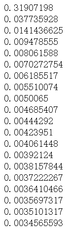
import numpy as np
 
x_data = np.linspace(-1,1,300)[:,np.newaxis]
noise = np.random.normal(0,0.05,x_data.shape).astype(np.float32)
y_data = np.square(x_data) - 0.5 + noise
 
# 利用占位符定义我们所需的神经网络的输入。 tf.placeholder()就是代表占位符，这里的None代表无论输入有多少都可以，因为输入只有一个特征，所以这里是1。
with tf.name_scope('inputs'):
    xs = tf.placeholder(tf.float32,[None,1],name='x_input')
    ys = tf.placeholder(tf.float32,[None,1],name='y_input')
 
#层
l1 = add_layer(xs,1,10,activation_function=tf.nn.relu)
prediction = add_layer(l1,10,1,activation_function=None)
 
#loss
loss = tf.reduce_mean(tf.reduce_sum(tf.square(ys-prediction),
                     reduction_indices=1))
 
#优化器
train_step = tf.train.GradientDescentOptimizer(learning_rate=0.1).minimize(loss)
 
# init = tf.initialize_all_variables() # tf 马上就要废弃这种写法
init = tf.global_variables_initializer()  # 替换成这样就好
sess = tf.Session()
sess.run(init)
 
for i in range(1000):
    sess.run(train_step,feed_dict={xs:x_data,ys:y_data})
    if i % 50 == 0:
    # to see the step improvement
        print(sess.run(loss, feed_dict={xs: x_data, ys: y_data}))

结果如下：

6. 结果可视化

import matplotlib.pyplot as plt
fig = plt.figure()
ax = fig.add_subplot(1,1,1)
ax.scatter(x_data,y_data)
# plt.ion() #plt.ion()用于连续显示
# plt.show()
 
 
# 每隔50次训练刷新一次图形，用红色、宽度为5的线来显示我们的预测数据和输入之间的关系，并暂停0.1s。
 
for i in range(1000):
    sess.run(train_step,feed_dict={xs:x_data,ys:y_data})
    if i % 50 == 0:
        try:
            ax.lines.remove(lines[0])
        except Exception:
            pass
        prediction_value = sess.run(prediction,feed_dict={xs:x_data})
        lines = ax.plot(x_data,prediction_value,'r-',lw=5)#线宽度=5
#         ax.lines.remove(lines[0])#去除lines的第一个线段
        plt.pause(0.1) #暂停0.1s
#         plt.show()

7. TensorFlow的优化器

tf.train.GradientDescentOptimizer
tf.train.AdadeltaOptimizer
tf.train.AdagradDAOptimizer
tf.train.MomentumOptimizer
tf.train.AdamOptimizer
tf.train.FtrlOptimizer
tf.train.RMSPropOptimizer

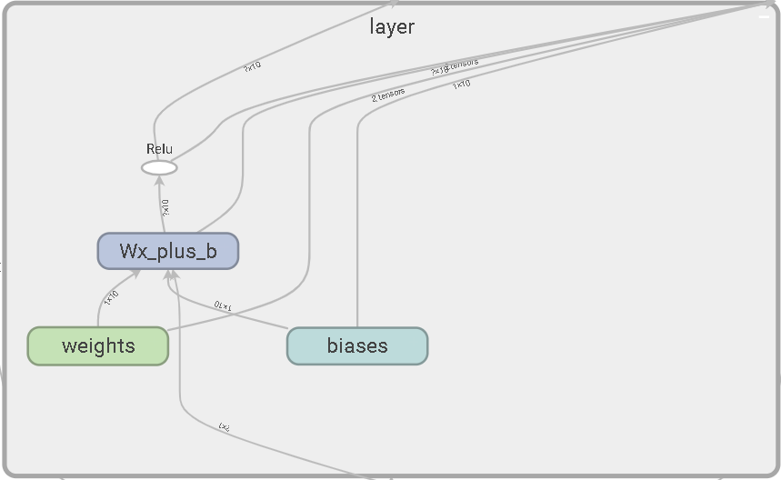
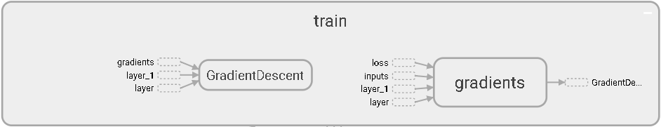
8. 可视化神经网络

# 图纸搭建   指定这里名称的会将来在可视化的图层inputs中显示出来
import tensorflow as tf
with tf.name_scope('inputs'):
    # define placeholder for inputs to network
    xs = tf.placeholder(tf.float32,[None,1],name='x_in')
    ys = tf.placeholder(tf.float32,[None,1],name='y_in')
 
def add_layer(inputs, in_size, out_size, activation_function=None):
    # add one more layer and return the output of this layer
    with tf.name_scope('layer'):
        with tf.name_scope('weights'):
            Weights = tf.Variable(
            tf.random_normal([in_size, out_size],name='W'), 
            name='W')
        with tf.name_scope('biases'):
            biases = tf.Variable(tf.zeros([1, out_size]) + 0.1,name='b')
        with tf.name_scope('Wx_plus_b'):
            Wx_plus_b = tf.add(
            tf.matmul(inputs, Weights), 
            biases)
        if activation_function is None:
            outputs = Wx_plus_b
        else:
            outputs = activation_function(Wx_plus_b, )
        return outputs
 
#层
l1 = add_layer(xs,1,10,activation_function=tf.nn.relu)
prediction = add_layer(l1,10,1,activation_function=None)
 
# the error between prediciton and real data
with tf.name_scope('loss'):
    loss = tf.reduce_mean(
    tf.reduce_sum(
    tf.square(ys - prediction),
#     eduction_indices=[1]
    ))
 
with tf.name_scope('train'):
    train_step = tf.train.GradientDescentOptimizer(0.1).minimize(loss)
 
sess = tf.Session() # get session
# tf.train.SummaryWriter soon be deprecated, use following
writer = tf.summary.FileWriter("E:/logs", sess.graph)
sess.run(tf.global_variables_initializer())

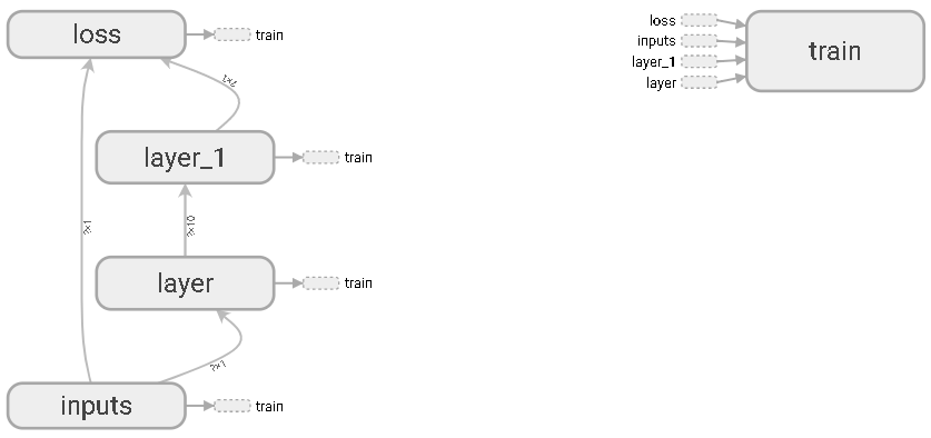
inputs输入层

隐藏层layer

隐藏层layer1

损失函数

训练

9. 可视化训练过程

输入数据：

import tensorflow as tf
import numpy as np
 
# 图纸搭建   指定这里名称的会将来在可视化的图层inputs中显示出来
with tf.name_scope('inputs'):
    # define placeholder for inputs to network
    xs = tf.placeholder(tf.float32,[None,1],name='x_in')
    ys = tf.placeholder(tf.float32,[None,1],name='y_in')
 
 ## make up some data
 x_data= np.linspace(-1, 1, 300, dtype=np.float32)[:,np.newaxis]
 noise=  np.random.normal(0, 0.05, x_data.shape).astype(np.float32)
 y_data= np.square(x_data) -0.5+ noise

添加层：

def add_layer(inputs , 
              in_size, 
              out_size,n_layer, 
              activation_function=None):
    ## add one more layer and return the output of this layer
    layer_name='layer%s'%n_layer
    with tf.name_scope(layer_name):
         with tf.name_scope('weights'):
              Weights= tf.Variable(tf.random_normal([in_size, out_size]),name='W')
              # tf.histogram_summary(layer_name+'/weights',Weights)
              tf.summary.histogram(layer_name + '/weights', Weights) # tensorflow >= 0.12
 
         with tf.name_scope('biases'):
              biases = tf.Variable(tf.zeros([1,out_size])+0.1, name='b')
              # tf.histogram_summary(layer_name+'/biase',biases)
              tf.summary.histogram(layer_name + '/biases', biases)  # Tensorflow >= 0.12
 
         with tf.name_scope('Wx_plus_b'):
              Wx_plus_b = tf.add(tf.matmul(inputs,Weights), biases)
 
         if activation_function is None: #最后一层不需要激活
            outputs=Wx_plus_b
         else:
            outputs= activation_function(Wx_plus_b)
 
         # tf.histogram_summary(layer_name+'/outputs',outputs)
         tf.summary.histogram(layer_name + '/outputs', outputs) # Tensorflow >= 0.12
 
    return outputs

损失函数：

with tf.name_scope('loss'):
     loss= tf.reduce_mean(tf.reduce_sum(
              tf.square(ys- prediction), reduction_indices=[1]))
     # tf.scalar_summary('loss',loss) # tensorflow < 0.12
     tf.summary.scalar('loss', loss) # tensorflow >= 0.12

接下来，开始合并打包。 tf.merge_all_summaries()方法会对我们所有的summaries合并到一起。因此在原有代码片段中添加：　　

sess= tf.Session()
 
# merged= tf.merge_all_summaries()    # tensorflow < 0.12
merged = tf.summary.merge_all() # tensorflow >= 0.12
 
# writer = tf.train.SummaryWriter('logs/', sess.graph)    # tensorflow < 0.12
writer = tf.summary.FileWriter("logs/", sess.graph) # tensorflow >=0.12
 
# sess.run(tf.initialize_all_variables()) # tf.initialize_all_variables() # tf 马上就要废弃这种写法
sess.run(tf.global_variables_initializer())  # 替换成这样就好

训练

for i in range(1000):
    sess.run(train_step,feed_dict={xs:x_data,ys:y_data})
    if i % 50 == 0:
        result = sess.run(merged,feed_dict={xs:x_data,ys:y_data})
    writer.add_summary(result,i)

（1）DISTRIBUTIONS

（2）EVENTS

1 2	`# tf.scalar_summary('loss',loss) # tensorflow < 0.12` `tf.summary.scalar('loss', loss)` `# tensorflow >= 0.12`

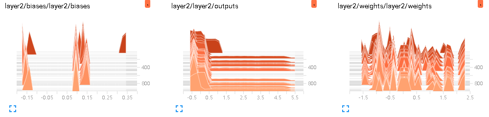
（3）HISTOGRAMS

1 2	`# tf.histogram_summary(layer_name+'/biase',biases) # Tensorflow < 0.12` `tf.summary.histogram(layer_name` `+` `'/biases', biases)` `# Tensorflow >= 0.12`