AlexNet—论文分析及复现

AlexNet卷积神经网络是由Alex Krizhevsky等人在2012年的ImagNet图像识别大赛获得冠军的一个卷积神经网络，该网络放到现在相对简单，但也是深度学习不错的卷积神经网络。论文：《ImageNet Classification with Deep Convolutional Neural Networks》

论文结构

Abstruct：简单介绍了AlexNet的结构及其成果
Introduction：神经网络要是有更快的GPU和更大的数据集我们的结果就会得到改善
The Dataset：介绍ILSVRC-2010和ImageNet数据集
The Architecture：ReLU非线性函数介绍、两个GPU进行训练、局部响应归一化、 Overlapping Pooling、整体架构
Reducing Overfitting：对抗过度拟合的方法,数据增强和Dropout
Details of learning：超参数的设置，权重及偏置的初始化
Results：介绍了AlexNet在比赛中获得的成果，性能评估（Qualitative Evaluations）：显示预测正确的概率，同一类的图像特征的欧式距离更近
Discussion：结果有了很大的改善，但是在某些方面还是有很多工作要做

AlexNet卷积神经网络的特点

1.非线性激活函数ReLu

在AlexNet出现之前，sigmoid是最为常用的非线性激活函数。sigmoid函数能够把输入的连续实值压缩到0和1之间。但是，它的缺点也非常明显：当神经网络层数过多或输入值非常大或者非常小的时候会出现饱和现象，即这些神经元的梯度接近0，因此存在梯度消失问题。

f (x) = \frac{1}{1 + e^{- x}}

$f(x)=\frac{1}{1+e^{-x}}$

图像代码：

 import numpy as np
import matplotlib.pyplot as plt
 
def sigmoid(x):
    return 1/(1+np.exp(-x))
 
x=np.arange(-5.0,5.0,0.1)
y=sigmoid(x)
plt.plot(x,y)
plt.ylim(-0.1,1.1)
plt.show()

图像：

tanh函数（双曲正切激活函数）很像是sigmoid函数的放大版。在实际使用中要略微优于sigmoid函数，因为它解决的中心对称问题。指数的计算复杂，计算成本高。梯度消失（梯度弥散）的特点依旧保留，因为两边的饱和性使得梯度消失，进而难以训练。

f (x) = \frac{e^{x} - e^{- x}}{e^{x} + e^{- x}}

$f(x)=\frac{e^{x}-e^{-x}}{e^{x}+e^{-x}}$

图像代码：

 import numpy as np
import matplotlib.pyplot as plt
 
def tanh(x):
    return (np.exp(x)-np.exp(-x))/(np.exp(x)+np.exp(-x))
 
x=np.arange(-5.0,5.0,0.1)
y=tanh(x)
plt.plot(x,y)
plt.show()

图像：

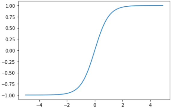
具体来说ReLU的好处有以下几点：

1.可以使神经网络训练更快

相比较于sigmoid和tanh，relu的求导速度更快

2.增加神经网络的非线性

ReLU是非线性函数

f (x) = m a x (0, x)

$f(x)=max(0,x)$

图像代码：

 import numpy as np
import matplotlib.pyplot as plt
 
def relu(x):
    return np.maximum(0,x)
 
x=np.arange(-5.0,5.0,0.1)
y=relu(x)
plt.plot(x,y)
plt.show()

图像：

3.使神经网络具有稀疏性

可以使一些神经元输出为0，可以增加网络的稀疏性

4.防止梯度消失

当数值过大或者过小时，sigmoid, tanh导数接近0，会导致方向传播时梯度消失的问题，relu为非饱和激活函数不存在此问题

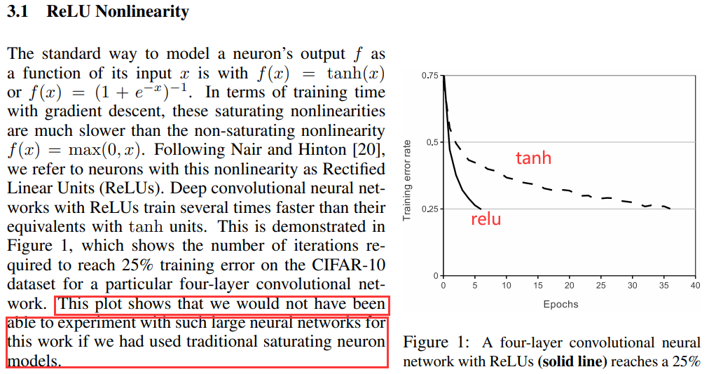
该图表明，如果我们使用传统的饱和神经元模型，我们将无法进行有如此大的神经网络的实验

2.Local Response Normalization(局部响应归一化)

局部响应归一化(local response normalization，LRN)的思想来源于生物学中的“侧抑制”，是指被激活的神经元抑制相邻的神经元。采用LRN的目的是，将数据分布调整到合理的范围内，便于计算处理，从而提高泛化能力。在神经网络中，我们用激活函数将神经元的输出做一个非线性映射，但是tanh和sigmoid这些传统的激活函数的值域都是有范围的，但是ReLU激活函数得到的值域没有一个区间，可以在[ 0 , ∞ ]，所以要对ReLU得到的结果进行归一化。简单理解，就是将利用当前第i个kernel的相邻n − 1个kernel对应(x,y) 的值来做归一化。论文中也给出了公式及介绍：

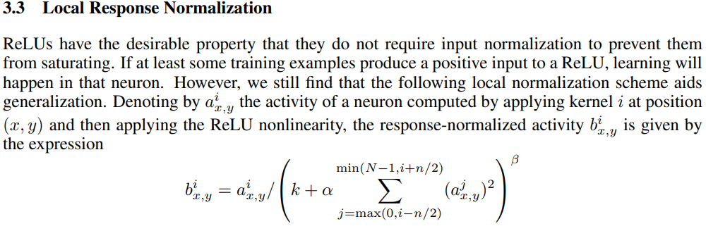
在2015年 Very Deep Convolutional Networks for Large-Scale Image Recognition.提到LRN基本没什么用，故这里不做叙述。

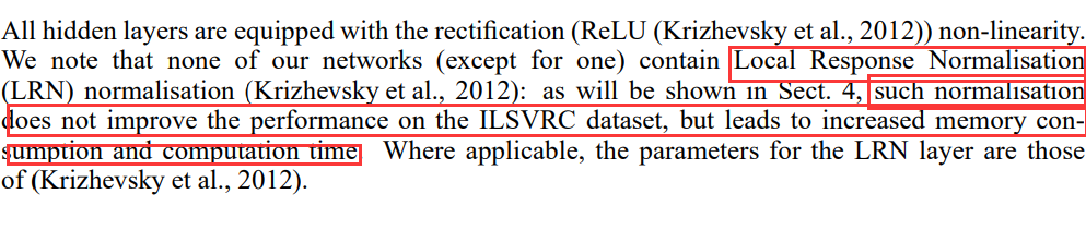
在后来出现的一些CNN架构模型中LRN已不再使用，因为出现了更有说服力的归一化——批量归一化，即BN。

3.两个GPU同时训练

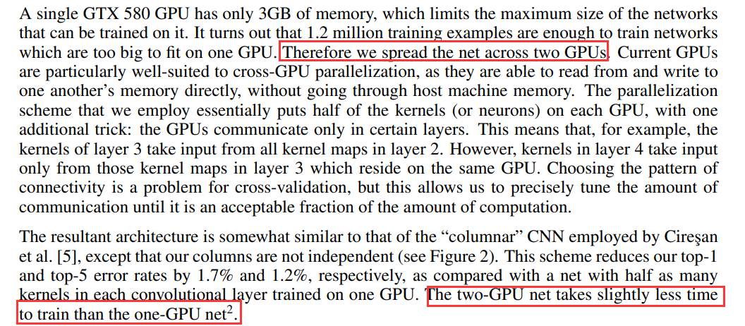
经过上述可知，两 GPU 网络的训练时间比单 GPU 网络略短。

4.Overlapping Pooling（重叠池化）

相对于传统的no-overlapping pooling，采用Overlapping Pooling不仅可以提升预测精度，同时一定程度上可以减缓过拟合

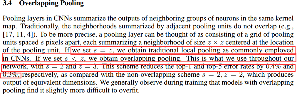
相比于正常池化（步长s=2，窗口z=2）重叠池化(步长s=2，窗口z=3) 可以减少top-1, top-5分别为0.4% 和0.3%；重叠池化可以避免过拟合。

5.Data Augmentation（数据增强）

论文中提到了两种形式的Data Augmentation

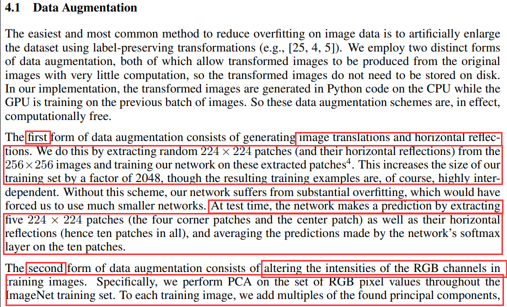
随机地从256 × 256的原始图像中截取224 × 224大小的区域（以及水平翻转的镜像），相当于增加了 $2×(256-224)^{2}=2048$ 倍的数据量,大大减轻过拟合，提升泛化能力。在进行测试的时候，取图片的四个角加中间一共5个位置，并进行左右翻转，一共获得10张图片，对他们在softmax层进行10次预测结果并求均值。

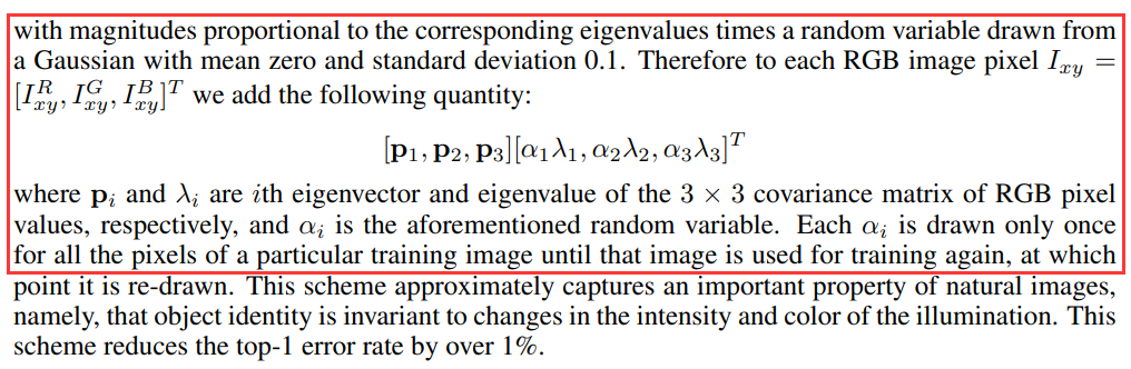
对图像的RGB数据进行PCA处理，并对主成分做一个标准差为0.1的高斯扰动，增加一些噪声，可以让错误率再下降1%。其中 pi 和 λi 是 RGB 像素值的 3 × 3 协方差矩阵的第 i 个特征向量和特征值，对于特定训练图像的所有像素，每个 αi 仅绘制一次，直到该图像再次用于训练，此时将重新绘制它。

6.Dropout

dropout可以让模型训练时，随机让网络上的一些节点失效（输出置零），此时的权重值不会更新，但会保存下来，因为这个过程只是对于本次训练。

通常会给dropout设置一个比率为p，也就是说每个节点都有p的概率将会失效，这种技术减少了神经元的复杂协同适应，因为一个神经元不能依赖于特定其他神经元的存在。

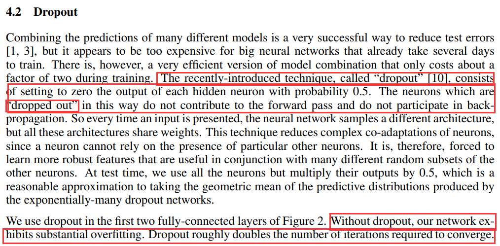
如果没有 dropout，我们的网络将表现出严重的过拟合。

AlexNet网络结构

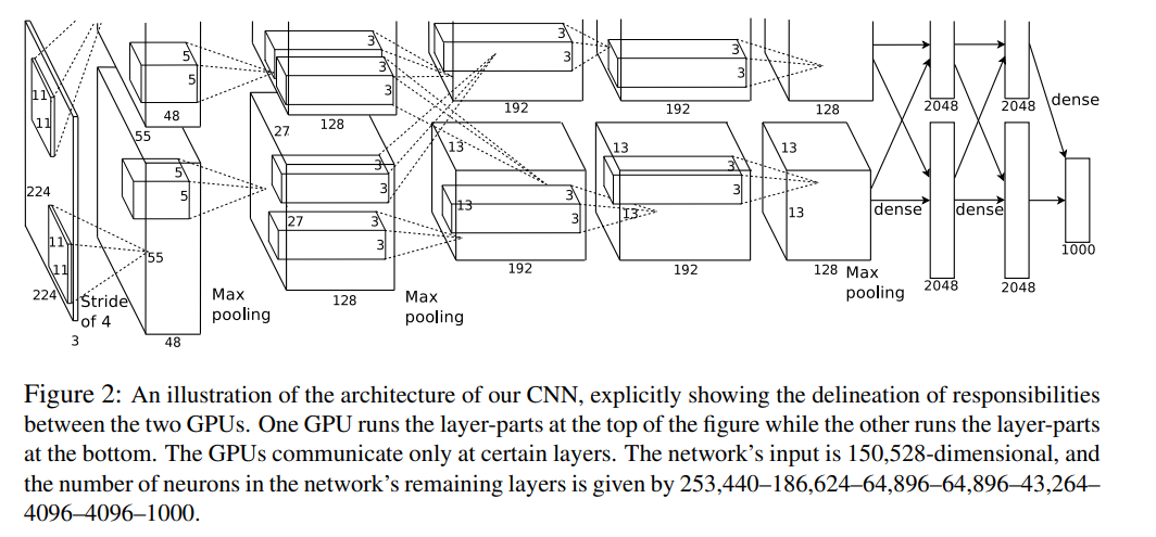
第一层卷积

原论文中，AlexNet的输入图像尺寸是224x224x3。但是实际图像尺寸为227x227x3，具体原因就不深究了，反正224x224x3不能推，227x227x3可以推。

第一个卷积层为11x11x3，即卷积核尺寸为11x11,有96个卷积核,步长为4,卷积层后紧跟ReLU,因此输出的尺寸为（227-11）/4+1=55,因此其输出的每个特征图为 55x55x96,同时后面经过LRN层处理,尺寸不变。

最大池化层,池化核大小为3x3,步长为2,输出的尺寸为（55-3）/2+1=27，因此特征图的大小为:27x27x96。由于双gpu处理，故每组数据有27x27x48个特征图，共两组数据，分别在两个gpu中进行运算。

第二层卷积

每组输入的数据为27x27x48，共两组数据，在两个GPU上训练

每组数据都被128个卷积核大小为: 5x5x48进行卷积运算,步长为1,尺寸不会改变,同样紧跟ReLU,和LRN层进行处理

最大池化层,池化核大小为3x3,步长为2,因此输出两组特征图:13x13x128

第三——五层卷积

输入的数据为13x13x128，共两组，分别在两个GPU上

第三层每组数据都被尺寸为 3x3x192的卷积核进行卷积运算,步长为1,加上ReLU，得到两组13x13x192的像素层

第四层经过padding=1填充后，每组数据都被尺寸大小为 3x3x192的卷积核卷积运算,步长为1,加上ReLU，输出两组13x13x192的像素层

第五层经过padding=1填充后，每组数据都被尺寸大小为 3x3x128的卷积核进行卷积运算,步长为1,加上ReLU，输出两组13x13x128的像素层

经过3x3池化窗口，步长为2，池化后输出两组6x6x256的像素层

第六——八层全连接层

第六层：4096 个神经元+ ReLU
第七层：4096个神经元 + ReLU
第八层：1000 个神经元，最后一层为softmax为1000类的概率值

实现代码

采用的数据集为Fashion-MNIST，数据集地址为：Fashion-MNIST

利用tensorflow对AlexNet神经网络进行简易实现

 import tensorflow as tf
import numpy as np
 
 
# 加载数据
class DataLoader():
    def __init__(self):
        fashion_mnist = tf.keras.datasets.fashion_mnist
        (self.train_images, self.train_labels), (self.test_images, self.test_labels) = fashion_mnist.load_data()
        self.train_images = np.expand_dims(self.train_images.astype(np.float32)/255.0,axis=-1)
        self.test_images = np.expand_dims(self.test_images.astype(np.float32)/255.0,axis=-1)
        self.train_labels = self.train_labels.astype(np.int32)
        self.test_labels = self.test_labels.astype(np.int32)
        self.num_train, self.num_test = self.train_images.shape[0], self.test_images.shape[0]
 
    def get_batch_train(self, batch_size):
        index = np.random.randint(0, np.shape(self.train_images)[0], batch_size)
        #need to resize images to (224,224)
        resized_images = tf.image.resize_with_pad(self.train_images[index],224,224,)
        return resized_images.numpy(), self.train_labels[index]
 
    def get_batch_test(self, batch_size):
        index = np.random.randint(0, np.shape(self.test_images)[0], batch_size)
        #need to resize images to (224,224)
        resized_images = tf.image.resize_with_pad(self.test_images[index],224,224,)
        return resized_images.numpy(), self.test_labels[index]
        
dataLoader = DataLoader()
 
 
# 搭建模型
net = tf.keras.models.Sequential([
    tf.keras.layers.Conv2D(filters=96,kernel_size=11,strides=4,activation='relu'),
    tf.keras.layers.BatchNormalization(),
    tf.keras.layers.MaxPool2D(pool_size=3, strides=2),
    tf.keras.layers.Conv2D(filters=256,kernel_size=5,padding='same',activation='relu'),
    tf.keras.layers.BatchNormalization(),
    tf.keras.layers.MaxPool2D(pool_size=3, strides=2),
    tf.keras.layers.Conv2D(filters=384,kernel_size=3,padding='same',activation='relu'),
    tf.keras.layers.Conv2D(filters=384,kernel_size=3,padding='same',activation='relu'),
    tf.keras.layers.Conv2D(filters=256,kernel_size=3,padding='same',activation='relu'),
    tf.keras.layers.MaxPool2D(pool_size=3, strides=2),
    tf.keras.layers.Flatten(),
    tf.keras.layers.Dense(4096,activation='relu'),
    tf.keras.layers.Dropout(0.5),
    tf.keras.layers.Dense(4096,activation='relu'),
    tf.keras.layers.Dropout(0.5),
    tf.keras.layers.Dense(10,activation='sigmoid')
])
 
 
# 超参数
batch_size = 128
learning_rate = 0.01
momentum=0.0
epoch=20
checkpoint = 20
 
 
# 训练
def train_alexnet():
    num_iter = dataLoader.num_train//batch_size
    for e in range(epoch):
        for n in range(num_iter):
            x_batch, y_batch = dataLoader.get_batch_train(batch_size)
            net.fit(x_batch, y_batch)
            if n%checkpoint == 0:
                net.save_weights("alexnet_weights.h5")
                
optimizer = tf.keras.optimizers.SGD(learning_rate=learning_rate, momentum=momentum, nesterov=False)
 
net.compile(optimizer=optimizer,
              loss='sparse_categorical_crossentropy',
              metrics=['accuracy'])
 
 
train_alexnet()
 
 
# 加载并评估
net.load_weights("alexnet_weights.h5")
x_test, y_test = dataLoader.get_batch_test(2000)
net.evaluate(x_test, y_test, verbose=2)

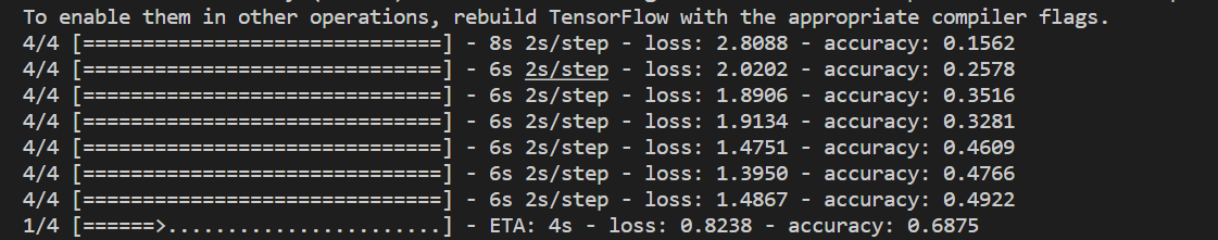
运行中：

比较详细的代码：

 # -*- coding=UTF-8 -*-  
import tensorflow as tf  
# 输入数据  
import input_data
 
  
mnist = input_data.read_data_sets("/tmp/data/", one_hot=True)  
# 定义网络超参数  
learning_rate = 0.001  
training_iters = 200000  
batch_size = 64  
display_step = 20  
# 定义网络参数  
n_input = 784  # 输入的维度  
n_classes = 10 # 标签的维度  
dropout = 0.8  # Dropout 的概率  
# 占位符输入  
x = tf.placeholder(tf.types.float32, [None, n_input])  
y = tf.placeholder(tf.types.float32, [None, n_classes])  
keep_prob = tf.placeholder(tf.types.float32)  
# 卷积操作  
def conv2d(name, l_input, w, b):  
    return tf.nn.relu(tf.nn.bias_add( \  
    tf.nn.conv2d(l_input, w, strides=[1, 1, 1, 1], padding='SAME'),b) \  
    , name=name)  
# 最大下采样操作  
def max_pool(name, l_input, k):  
    return tf.nn.max_pool(l_input, ksize=[1, k, k, 1], \  
    strides=[1, k, k, 1], padding='SAME', name=name)  
# 归一化操作  
def norm(name, l_input, lsize=4):  
    return tf.nn.lrn(l_input, lsize, bias=1.0, alpha=0.001 / 9.0, beta=0.75, name=name)  
# 定义整个网络   
def alex_net(_X, _weights, _biases, _dropout):  
    _X = tf.reshape(_X, shape=[-1, 28, 28, 1]) # 向量转为矩阵  
    # 卷积层  
    conv1 = conv2d('conv1', _X, _weights['wc1'], _biases['bc1'])  
    # 下采样层  
    pool1 = max_pool('pool1', conv1, k=2)  
    # 归一化层  
    norm1 = norm('norm1', pool1, lsize=4)  
    # Dropout  
    norm1 = tf.nn.dropout(norm1, _dropout)  
   
    # 卷积  
    conv2 = conv2d('conv2', norm1, _weights['wc2'], _biases['bc2'])  
    # 下采样  
    pool2 = max_pool('pool2', conv2, k=2)  
    # 归一化  
    norm2 = norm('norm2', pool2, lsize=4)  
    # Dropout  
    norm2 = tf.nn.dropout(norm2, _dropout)  
   
    # 卷积  
    conv3 = conv2d('conv3', norm2, _weights['wc3'], _biases['bc3'])  
    # 下采样  
    pool3 = max_pool('pool3', conv3, k=2)  
    # 归一化  
    norm3 = norm('norm3', pool3, lsize=4)  
    # Dropout  
    norm3 = tf.nn.dropout(norm3, _dropout)  
   
    # 全连接层，先把特征图转为向量  
    dense1 = tf.reshape(norm3, [-1, _weights['wd1'].get_shape().as_list()[0]])   
    dense1 = tf.nn.relu(tf.matmul(dense1, _weights['wd1']) + _biases['bd1'], name='fc1')   
    # 全连接层  
    dense2 = tf.nn.relu(tf.matmul(dense1, _weights['wd2']) + _biases['bd2'], name='fc2') 
    # Relu activation  
    # 网络输出层  
    out = tf.matmul(dense2, _weights['out']) + _biases['out']  
    return out  
   
# 存储所有的网络参数  
weights = {  
    'wc1': tf.Variable(tf.random_normal([3, 3, 1, 64])),  
    'wc2': tf.Variable(tf.random_normal([3, 3, 64, 128])),  
    'wc3': tf.Variable(tf.random_normal([3, 3, 128, 256])),  
    'wd1': tf.Variable(tf.random_normal([4*4*256, 1024])),  
    'wd2': tf.Variable(tf.random_normal([1024, 1024])),  
    'out': tf.Variable(tf.random_normal([1024, 10]))  
}  
biases = {  
    'bc1': tf.Variable(tf.random_normal([64])),  
    'bc2': tf.Variable(tf.random_normal([128])),  
    'bc3': tf.Variable(tf.random_normal([256])),  
    'bd1': tf.Variable(tf.random_normal([1024])),  
    'bd2': tf.Variable(tf.random_normal([1024])),  
    'out': tf.Variable(tf.random_normal([n_classes]))  
}  
# 构建模型  
pred = alex_net(x, weights, biases, keep_prob)  
# 定义损失函数和学习步骤  
cost = tf.reduce_mean(tf.nn.softmax_cross_entropy_with_logits(pred, y))  
optimizer = tf.train.AdamOptimizer(learning_rate=learning_rate).minimize(cost)  
# 测试网络  
correct_pred = tf.equal(tf.argmax(pred,1), tf.argmax(y,1))  
accuracy = tf.reduce_mean(tf.cast(correct_pred, tf.float32))  
# 初始化所有的共享变量  
init = tf.initialize_all_variables()  
# 开启一个训练  
with tf.Session() as sess:  
    sess.run(init)  
    step = 1  
    # Keep training until reach max iterations  
    while step * batch_size < training_iters:  
        batch_xs, batch_ys = mnist.train.next_batch(batch_size)  
        # 获取批数据  
        sess.run(optimizer, feed_dict={x: batch_xs, y: batch_ys, keep_prob: dropout})  
        if step % display_step == 0:  
            # 计算精度  
            acc = sess.run(accuracy, feed_dict={x: batch_xs, y: batch_ys, keep_prob: 1.})  
            # 计算损失值  
            loss = sess.run(cost, feed_dict={x: batch_xs, y: batch_ys, keep_prob: 1.})  
            print "Iter " + str(step*batch_size) + ", Minibatch Loss= " + "{:.6f}".format(loss) + ", Training Accuracy= " + "{:.5f}".format(acc)  
        step += 1  
    print "Optimization Finished!"  
    # 计算测试精度  
    print "Testing Accuracy:", sess.run(accuracy, feed_dict={x: mnist.test.images[:256], y: mnist.test.labels[:256], keep_prob: 1.})  
 
# 以上代码忽略了部分卷积层，全连接层使用了特定的权重。

注：此来源于百度，仅供学习参考

参考文献：

《ImageNet Classification with Deep Convolutional Neural Networks》

本文写于2022年7月27日00:41

posted @ 2022-07-28 10:53 NGIWS 阅读(2285) 评论(2) 编辑收藏举报

刷新页面返回顶部

登录后才能查看或发表评论，立即登录或者逛逛博客园首页

相关博文：

· 梯度下降算法实现原理(Gradient Descent)

· 机器学习-感知机模型

· 【论文笔记】AlexNet

· 深度卷积神经网络（AlexNet）

· AlexNet文献阅读与代码实现

阅读排行：
· 阿里巴巴 QwQ-32B真的超越了 DeepSeek R-1吗？
· 10年+ .NET Coder 心语 ── 封装的思维：从隐藏、稳定开始理解其本质意义
· 【设计模式】告别冗长if-else语句：使用策略模式优化代码结构
· 字符编码：从基础到乱码解决
· 提示词工程——AI应用必不可少的技术

公告

昵称： NGIWS
园龄： 3年5个月
粉丝： 22
关注： 0

+加关注

2025年3月

日

一

二

三

四

五

六

NGIWS

AlexNet—论文分析及复现

论文结构

AlexNet卷积神经网络的特点

1.非线性激活函数ReLu

具体来说ReLU的好处有以下几点：

2.Local Response Normalization(局部响应归一化)

3.两个GPU同时训练

4.Overlapping Pooling（重叠池化）

5.Data Augmentation（数据增强）

6.Dropout

AlexNet网络结构

实现代码

公告

搜索

常用链接

积分与排名

随笔档案

阅读排行榜

推荐排行榜

	import numpy as np
	import matplotlib.pyplot as plt

	def sigmoid(x):
	return 1/(1+np.exp(-x))

	x=np.arange(-5.0,5.0,0.1)
	y=sigmoid(x)
	plt.plot(x,y)
	plt.ylim(-0.1,1.1)
	plt.show()

	import numpy as np
	import matplotlib.pyplot as plt

	def tanh(x):
	return (np.exp(x)-np.exp(-x))/(np.exp(x)+np.exp(-x))

	x=np.arange(-5.0,5.0,0.1)
	y=tanh(x)
	plt.plot(x,y)
	plt.show()

	import numpy as np
	import matplotlib.pyplot as plt

	def relu(x):
	return np.maximum(0,x)

	x=np.arange(-5.0,5.0,0.1)
	y=relu(x)
	plt.plot(x,y)
	plt.show()

	import tensorflow as tf
	import numpy as np


	# 加载数据
	class DataLoader():
	def __init__(self):
	fashion_mnist = tf.keras.datasets.fashion_mnist
	(self.train_images, self.train_labels), (self.test_images, self.test_labels) = fashion_mnist.load_data()
	self.train_images = np.expand_dims(self.train_images.astype(np.float32)/255.0,axis=-1)
	self.test_images = np.expand_dims(self.test_images.astype(np.float32)/255.0,axis=-1)
	self.train_labels = self.train_labels.astype(np.int32)
	self.test_labels = self.test_labels.astype(np.int32)
	self.num_train, self.num_test = self.train_images.shape[0], self.test_images.shape[0]

	def get_batch_train(self, batch_size):
	index = np.random.randint(0, np.shape(self.train_images)[0], batch_size)
	#need to resize images to (224,224)
	resized_images = tf.image.resize_with_pad(self.train_images[index],224,224,)
	return resized_images.numpy(), self.train_labels[index]

	def get_batch_test(self, batch_size):
	index = np.random.randint(0, np.shape(self.test_images)[0], batch_size)
	#need to resize images to (224,224)
	resized_images = tf.image.resize_with_pad(self.test_images[index],224,224,)
	return resized_images.numpy(), self.test_labels[index]

	dataLoader = DataLoader()


	# 搭建模型
	net = tf.keras.models.Sequential([
	tf.keras.layers.Conv2D(filters=96,kernel_size=11,strides=4,activation='relu'),
	tf.keras.layers.BatchNormalization(),
	tf.keras.layers.MaxPool2D(pool_size=3, strides=2),
	tf.keras.layers.Conv2D(filters=256,kernel_size=5,padding='same',activation='relu'),
	tf.keras.layers.BatchNormalization(),
	tf.keras.layers.MaxPool2D(pool_size=3, strides=2),
	tf.keras.layers.Conv2D(filters=384,kernel_size=3,padding='same',activation='relu'),
	tf.keras.layers.Conv2D(filters=384,kernel_size=3,padding='same',activation='relu'),
	tf.keras.layers.Conv2D(filters=256,kernel_size=3,padding='same',activation='relu'),
	tf.keras.layers.MaxPool2D(pool_size=3, strides=2),
	tf.keras.layers.Flatten(),
	tf.keras.layers.Dense(4096,activation='relu'),
	tf.keras.layers.Dropout(0.5),
	tf.keras.layers.Dense(4096,activation='relu'),
	tf.keras.layers.Dropout(0.5),
	tf.keras.layers.Dense(10,activation='sigmoid')
	])


	# 超参数
	batch_size = 128
	learning_rate = 0.01
	momentum=0.0
	epoch=20
	checkpoint = 20


	# 训练
	def train_alexnet():
	num_iter = dataLoader.num_train//batch_size
	for e in range(epoch):
	for n in range(num_iter):
	x_batch, y_batch = dataLoader.get_batch_train(batch_size)
	net.fit(x_batch, y_batch)
	if n%checkpoint == 0:
	net.save_weights("alexnet_weights.h5")

	optimizer = tf.keras.optimizers.SGD(learning_rate=learning_rate, momentum=momentum, nesterov=False)

	net.compile(optimizer=optimizer,
	loss='sparse_categorical_crossentropy',
	metrics=['accuracy'])


	train_alexnet()


	# 加载并评估
	net.load_weights("alexnet_weights.h5")
	x_test, y_test = dataLoader.get_batch_test(2000)
	net.evaluate(x_test, y_test, verbose=2)

	# -- coding=UTF-8 --
	import tensorflow as tf
	# 输入数据
	import input_data


	mnist = input_data.read_data_sets("/tmp/data/", one_hot=True)
	# 定义网络超参数
	learning_rate = 0.001
	training_iters = 200000
	batch_size = 64
	display_step = 20
	# 定义网络参数
	n_input = 784 # 输入的维度
	n_classes = 10 # 标签的维度
	dropout = 0.8 # Dropout 的概率
	# 占位符输入
	x = tf.placeholder(tf.types.float32, [None, n_input])
	y = tf.placeholder(tf.types.float32, [None, n_classes])
	keep_prob = tf.placeholder(tf.types.float32)
	# 卷积操作
	def conv2d(name, l_input, w, b):
	return tf.nn.relu(tf.nn.bias_add( \
	tf.nn.conv2d(l_input, w, strides=[1, 1, 1, 1], padding='SAME'),b) \
	, name=name)
	# 最大下采样操作
	def max_pool(name, l_input, k):
	return tf.nn.max_pool(l_input, ksize=[1, k, k, 1], \
	strides=[1, k, k, 1], padding='SAME', name=name)
	# 归一化操作
	def norm(name, l_input, lsize=4):
	return tf.nn.lrn(l_input, lsize, bias=1.0, alpha=0.001 / 9.0, beta=0.75, name=name)
	# 定义整个网络
	def alex_net(_X, _weights, _biases, _dropout):
	_X = tf.reshape(_X, shape=[-1, 28, 28, 1]) # 向量转为矩阵
	# 卷积层
	conv1 = conv2d('conv1', _X, _weights['wc1'], _biases['bc1'])
	# 下采样层
	pool1 = max_pool('pool1', conv1, k=2)
	# 归一化层
	norm1 = norm('norm1', pool1, lsize=4)
	# Dropout
	norm1 = tf.nn.dropout(norm1, _dropout)

	# 卷积
	conv2 = conv2d('conv2', norm1, _weights['wc2'], _biases['bc2'])
	# 下采样
	pool2 = max_pool('pool2', conv2, k=2)
	# 归一化
	norm2 = norm('norm2', pool2, lsize=4)
	# Dropout
	norm2 = tf.nn.dropout(norm2, _dropout)

	# 卷积
	conv3 = conv2d('conv3', norm2, _weights['wc3'], _biases['bc3'])
	# 下采样
	pool3 = max_pool('pool3', conv3, k=2)
	# 归一化
	norm3 = norm('norm3', pool3, lsize=4)
	# Dropout
	norm3 = tf.nn.dropout(norm3, _dropout)

	# 全连接层，先把特征图转为向量
	dense1 = tf.reshape(norm3, [-1, _weights['wd1'].get_shape().as_list()[0]])
	dense1 = tf.nn.relu(tf.matmul(dense1, _weights['wd1']) + _biases['bd1'], name='fc1')
	# 全连接层
	dense2 = tf.nn.relu(tf.matmul(dense1, _weights['wd2']) + _biases['bd2'], name='fc2')
	# Relu activation
	# 网络输出层
	out = tf.matmul(dense2, _weights['out']) + _biases['out']
	return out

	# 存储所有的网络参数
	weights = {
	'wc1': tf.Variable(tf.random_normal([3, 3, 1, 64])),
	'wc2': tf.Variable(tf.random_normal([3, 3, 64, 128])),
	'wc3': tf.Variable(tf.random_normal([3, 3, 128, 256])),
	'wd1': tf.Variable(tf.random_normal([44256, 1024])),
	'wd2': tf.Variable(tf.random_normal([1024, 1024])),
	'out': tf.Variable(tf.random_normal([1024, 10]))
	}
	biases = {
	'bc1': tf.Variable(tf.random_normal([64])),
	'bc2': tf.Variable(tf.random_normal([128])),
	'bc3': tf.Variable(tf.random_normal([256])),
	'bd1': tf.Variable(tf.random_normal([1024])),
	'bd2': tf.Variable(tf.random_normal([1024])),
	'out': tf.Variable(tf.random_normal([n_classes]))
	}
	# 构建模型
	pred = alex_net(x, weights, biases, keep_prob)
	# 定义损失函数和学习步骤
	cost = tf.reduce_mean(tf.nn.softmax_cross_entropy_with_logits(pred, y))
	optimizer = tf.train.AdamOptimizer(learning_rate=learning_rate).minimize(cost)
	# 测试网络
	correct_pred = tf.equal(tf.argmax(pred,1), tf.argmax(y,1))
	accuracy = tf.reduce_mean(tf.cast(correct_pred, tf.float32))
	# 初始化所有的共享变量
	init = tf.initialize_all_variables()
	# 开启一个训练
	with tf.Session() as sess:
	sess.run(init)
	step = 1
	# Keep training until reach max iterations
	while step * batch_size < training_iters:
	batch_xs, batch_ys = mnist.train.next_batch(batch_size)
	# 获取批数据
	sess.run(optimizer, feed_dict={x: batch_xs, y: batch_ys, keep_prob: dropout})
	if step % display_step == 0:
	# 计算精度
	acc = sess.run(accuracy, feed_dict={x: batch_xs, y: batch_ys, keep_prob: 1.})
	# 计算损失值
	loss = sess.run(cost, feed_dict={x: batch_xs, y: batch_ys, keep_prob: 1.})
	print "Iter " + str(step*batch_size) + ", Minibatch Loss= " + "{:.6f}".format(loss) + ", Training Accuracy= " + "{:.5f}".format(acc)
	step += 1
	print "Optimization Finished!"
	# 计算测试精度
	print "Testing Accuracy:", sess.run(accuracy, feed_dict={x: mnist.test.images[:256], y: mnist.test.labels[:256], keep_prob: 1.})

	# 以上代码忽略了部分卷积层，全连接层使用了特定的权重。