MongoDB 操作

MongoDB 是一种流行的非关系型数据库，它提供了一种面向文档的数据存储方式。每
种商品就是集合中的一份文档。商品具有一些描述字段和一个数组类型的评论字段。所有
评论都是一个子文档，因此每个逻辑项都可以以自己的逻辑形式进行存储。
以下是集合中一种商品的 JSON（https://en.wikipedia.org/wiki/JSON）文件存储方式：
{
"code":"A0000001",
"name":"Product-A",
"type":"Type-I",
"price":29.5,
"amount":500,
"comments":[
{
"user":"david",
"score":8,
"text":"This is a good product"
},
{
"user":"jenny",
"score":5,
"text":"Just so so"
}
]
}
关系型数据库可能具有许多模式（schemas）。每种模式（或数据库）可以由多张表组
成，每张表可能含有多条记录。相似地，一个 MongoDB 实例可以搭建多个数据库。每个
数据库有可以存在多个集合，每个集合内可能有多个文档。二者的主要区别在于，关系型
数据库中，一张表的所有记录具有相同的结构，但 MongoDB 数据库集合内的文档却没有
模式限制，可以灵活地实现嵌套结构。
例如，前面的 JSON 格式用一个这样的文档描述一种商品的特征，文档内的 code、
name、type、price 和 amount 这些数据字段都是简单的数据类型，而 comment 则是
数组对象。每条评论由 comments 数组的一个对象所表示，该对象具有 user、
score 和 text 的结构。该商品的所有评论共同组成一个对象，并存储在 comments 字段
中。因此，根据商品的信息和评论，每种商品都是高度自包含的。如果我们需要某种产品
的信息，不必再连接两张表，只需选出几个字段即可。
安装 MongoDB，请访问 https://docs.mongodb.com/manual/installation/，根据说明操作即
可，它支持几乎所有主流平台。
1．用 MongoDB 查询数据
假设我们有一个在本地设备上运行的 MongoDB 实例，它使用 mongolite 扩展包操
作 MongoDB。可运行以下代码安装该扩展包：
install.packages("mongolite")
一旦安装好了扩展包，我们便可以通过声明集合、数据库和 MongoDB 的地址来创
建 Mongo 连接：
library(mongolite)
m <- mongo("products", "test", "mongodb://localhost")
首先，我们创建一个到本地的 MongoDB 实例的连接。初始状态下，集合 products 不
含任何文档。
m$count( )
## [1] 0
为了插入一个带评论的商品，直接将 JSON 文档以字符串形式传递给 m$insert( )：
m$insert('
{
"code": "A0000001",
"name": "Product-A",
"type": "Type-I",
"price": 29.5,
"amount": 500,
"comments": [
{
"user": "david",
"score": 8,
"text": "This is a good product"
},
{
"user": "jenny",
"score": 5,
"text": "Just so so"
}
]
}')
现在，这个集合中就有一个文档了：
m$count( )
## [1] 1
此外，也可以用 R 中的列表对象来表示相同的结构。以下代码使用 list( ) 插入了
第 2 个商品：
m$insert(list(
code = "A0000002",
name = "Product-B",
type = "Type-II",
price = 59.9,
amount = 200L,
comments = list(
list(user = "tom", score = 6L,
text = "Just fine"),
list(user = "mike", score = 9L,
text = "great product!")
)
), auto_unbox = TRUE)
注意，R 没有提供标量类型，默认情况下，所有向量在 MongoDB 中都会被解释
为 JSON 数组，除非设置 auto_unbox = TRUE，它会将单元素向量转换为 JSON 中的标
量。 如果没有设置 auto_unbox = TRUE，就要用 jsonlite::unbox( ) 来确保标量
输出或用 I( ) 确保数组输出。
现在，集合中有两个文档了：
m$count( )
## [1] 2
接着，我们用 m$find( ) 取出集合中的所有文档，为了更方便地进行数据处理，结
果会自动简化为数据框类型。
products <- m$find( )
##
Found 4 records...
Imported 4 records. Simplifying into dataframe...
str(products)
## 'data.frame': 4 obs. of 6 variables:
## $ code : chr "A0000001" "A0000002"
## $ name : chr "Product-A" "Product-B"
## $ type : chr "Type-I" "Type-II"
## $ price : num 29.5 59.9
## $ amount : int 500 200
## $ comments:List of 2
## ..$ :'data.frame': 2 obs. of 3 variables:
## .. ..$ user : chr "david" "jenny"
## .. ..$ score: int 8 5
## .. ..$ text : chr "This is a good product" "Just so so"
## ..$ :'data.frame': 2 obs. of 3 variables:
## .. ..$ user : chr "tom" "mike"
## .. ..$ score: int 6 9
## .. ..$ text : chr "Just fine" "great product!"
为了避免自动转换，可以用 m$iterate( ) 在集合中进行迭代，并得到具有原始存
储形式的列表对象：
iter <- m$iterate( )
products <- iter$batch(2)
str(products)
## List of 2
## $ :List of 6
## ..$ code : chr "A0000001"
## ..$ name : chr "Product-A"
## ..$ type : chr "Type-I"
## ..$ price : num 29.5
## ..$ amount : int 500
## ..$ comments:List of 2
## .. ..$ :List of 3
## .. .. ..$ user : chr "david"
## .. .. ..$ score: int 8
## .. .. ..$ text : chr "This is a good product"
## .. ..$ :List of 3
## .. .. ..$ user : chr "jenny"
## .. .. ..$ score: int 5
## .. .. ..$ text : chr "Just so so"
## $ :List of 6
## ..$ code : chr "A0000002"
## ..$ name : chr "Product-B"
## ..$ type : chr "Type-II"
## ..$ price : num 59.9
## ..$ amount : int 200
## ..$ comments:List of 2
## .. ..$ :List of 3
## .. .. ..$ user : chr "tom"
## .. .. ..$ score: int 6
## .. .. ..$ text : chr "Just fine"
## .. ..$ :List of 3
## .. .. ..$ user : chr "mike"
## .. .. ..$ score: int 9
## .. .. ..$ text : chr "great product!"
还可以在 m$find( ) 中声明条件查询及字段来筛选集合：
首先，我们查询 code 为 A0000001 的文档，并取出 name、price 和 amount
字段：
m$find('{ "code": "A0000001" }',
'{ "_id": 0, "name": 1, "price": 1, "amount": 1 }')
##
Found 2 records...
Imported 2 records. Simplifying into dataframe...
## name price amount
## 1 Product-A 29.5 500
然后，查询 price 字段大于等于 40 的文档，这一步可以通过条件查询的 $gte 运
算符来实现：
m$find('{ "price": { "$gte": 40 } }',
'{ "_id": 0, "name": 1, "price": 1, "amount": 1 }')
##
Found 1 records...
Imported 1 records. Simplifying into dataframe...
## name price amount
## 1 Product-B 59.9 200
## 2 Product-B 59.9 200
我们不仅可以查询文档字段，也可以查询数组字段中某个对象。下列代码用来取出对
应评论数组中评分为 9 分的商品文档：
m$find('{ "comments.score": 9 }',
'{ "_id": 0, "code": 1, "name": 1}')
##
Found 2 records...
Imported 2 records. Simplifying into dataframe...
## code name
## 1 A0000002 Product-B
类似地，下面的代码可取出 6 分以下的低分评论的商品文档：
m$find('{ "comments.score": { "$lt": 6 }}',
'{ "_id": 0, "code": 1, "name": 1}')
##
Found 2 records...
Imported 2 records. Simplifying into dataframe...
## code name
## 1 A0000001 Product-A
注意，使用 . 符号可以轻松实现访问子文档中的字段，这使我们能够更加灵活地对嵌
套结构进行控制：
## [1] TRUE
m$insert( ) 函数也可以用来处理 R 中的数据框。现在，创建一个新的 MongoDB 连
接，并连接至另一个集合：
m <- mongo("students", "test", "mongodb://localhost")
我们创建一个 MongoDB 连接对象 m，来处理本地 MongoDB 实例中 test 数据库
的 students 集合。
m$count( )
## [1] 0
最初，这个集合中没有文档。我们创建一个简单的数据框，以便向其中插入一些
数据：
students <- data.frame(
name = c("David", "Jenny", "Sara", "John"),
age = c(25, 23, 26, 23),
major = c("Statistics", "Physics", "Computer Science", "Statistics"),
projects = c(2, 1, 3, 1),
stringsAsFactors = FALSE
)
students
## name age major projects
## 1 David 25 Statistics 2
## 2 Jenny 23 Physics 1
## 3 Sara 26 Computer Science 3
## 4 John 23 Statistics 1
然后，将这些行行为文档插入到集合中：
m$insert(students)
##
Complete! Processed total of 4 rows.
现在，集合中有一些文档了：
m$count( )
## [1] 4
用 find( ) 取出所有的文档：
m$find( )
##
Found 4 records...
Imported 4 records. Simplifying into dataframe...
## name age major projects
## 1 David 25 Statistics 2
## 2 Jenny 23 Physics 1
## 3 Sara 26 Computer Science 3
## 4 John 23 Statistics 1
正如前面的例子中所提到的，文档存储在 MongoDB 集合中的方式，与关系型数据库
中字段存储在表中的方式是不同的。MongoDB 集合中的一个文档，更像是一个 JSON 文档，
但实际上，它是以二进制数据形式存储的，以获得高性能和紧凑性。m$find( ) 函数首
先取出类似 JSON 格式的数据，然后将它简化成便于处理的数据格式。
为了筛选数据，我们可以在 m$find( ) 中声明查询条件。例如，找出名为 Jenny 的
所有文档：
m$find('{ "name": "Jenny" }')
##
Found 1 records...
Imported 1 records. Simplifying into dataframe...
## name age major projects
## 1 Jenny 23 Physics 1
结果自动强制转换为数据框，以便于使用。然后，查询 projects 字段数值大于等于
2 的所有文档：
m$find('{ "projects": { "$gte": 2 }}')
##
Found 2 records...
Imported 2 records. Simplifying into dataframe...
## name age major projects
## 1 David 25 Statistics 2
## 2 Sara 26 Computer Science 3
为了选择字段，我们可以指定 find( ) 函数的 fields 参数：
m$find('{ "projects": { "$gte": 2 }}',
'{ "_id": 0, "name": 1, "major": 1 }')
##
Found 2 records...
Imported 2 records. Simplifying into dataframe...
## name major
## 1 David Statistics
## 2 Sara Computer Science
也可以设置 sort 参数来整理数据：
m$find('{ "projects": { "$gte": 2 }}',
fields ='{ "_id": 0, "name": 1, "age": 1 }',
sort ='{ "age": -1 }')
##
Found 2 records...
Imported 2 records. Simplifying into dataframe...
## name age
## 1 Sara 26
## 2 David 25
指定 limit 参数来限制返回文档的数量：
m$find('{ "projects": { "$gte": 2 }}',
fields ='{ "_id": 0, "name": 1, "age": 1 }',
sort ='{ "age": -1 }',
limit =1)
##
Found 1 records...
Imported 1 records. Simplifying into dataframe...
## name age
## 1 Sara 26
同样，我们可以得到所有文档中某一字段中所有不同的值：
m$distinct("major")
## [1] "Statistics" "Physics" "Computer Science"
得到基于某个条件的不同取值：
m$distinct("major", '{ "projects": { "$gte": 2 } }')
## [1] "Statistics" "Computer Science"
要更新某个文档，我们可以调用 update( )，找到所选文档，设置特定字段的取值：
m$update('{ "name": "Jenny" }', '{ "$set": { "age": 24 } }')
## [1] TRUE
m$find()
##
Found 4 records...
Imported 4 records. Simplifying into dataframe...
## name age major projects
## 1 David 25 Statistics 2
## 2 Jenny 24 Physics 1
## 3 Sara 26 Computer Science 3
## 4 John 23 Statistics 1
2．创建或移除索引
与关系型数据库类似，MongoDB 也支持索引。一个集合可以有多个索引，并且索引字
段被高速缓存在存储器中以便快速查找。适当地创建索引能够使文档检索变得非常高效。
借助 mongolite 扩展包能够轻松地在 MongoDB 中创建索引，这个工作在我们向集
合中导入数据之前或之后进行都是可行的。然而，如果在已经导入了数十亿的数据后，再
创建索引会是一件费时的工作。同样，如果在导入文档前就创建了许多索引，就会影响导
入集合的性能。
这里，我们为 students 集合创建一个索引：
m$index('{ "name": 1 }')
## v key._id key.name name ns
## 1 2 1 NA _id_ test.students
## 2 2 NA 1 name_1 test.students
现在，如果通过索引字段查找文档，其运算性能是优异的：
m$find('{ "name": "Sara" }')
##
Found 1 records...
Imported 1 records. Simplifying into dataframe...
## name age major projects
## 1 Sara 26 Computer Science 3
如果没有文档满足条件，则会返回一个空的数据框：
m$find('{ "name": "Jane" }')
##
Imported 0 records. Simplifying into dataframe...
## data frame with 0 columns and 0 rows
最后，使用 drop( ) 删除集合。
m$drop( )
## [1] TRUE
显然，如果数据量本身很小，那么由索引带来的性能提升是很有限的。在下一个例子
中，我们会创建一个有许多行的数据框，以便比较使用索引和不使用索引两种情况下，查
找文档的性能差异。
set.seed(123)
m <- mongo("simulation", "test")
sim_data <- expand.grid(
type = c("A", "B", "C", "D", "E"),
category = c("P-1", "P-2", "P-3"),
group = 1:20000,
stringsAsFactors = FALSE)
head(sim_data)
## type category group
## 1 A P-1 1
## 2 B P-1 1
## 3 C P-1 1
## 4 D P-1 1
## 5 E P-1 1
## 6 A P-2 1
索引字段已经创建好了。接下来，我们生成一些随机数字：
sim_data$score1 <- rnorm(nrow(sim_data), 10, 3)
sim_data$test1 <- rbinom(nrow(sim_data), 100, 0.8)
现在的数据框如下所示：
head(sim_data)
## type category group score1 test1
## 1 A P-1 1 8.318573 80
## 2 B P-1 1 9.309468 75
## 3 C P-1 1 14.676125 77
## 4 D P-1 1 10.211525 79
## 5 E P-1 1 10.387863 80
## 6 A P-2 1 15.145195 76
然后向 simulation 集合中插入以下数据：
m$insert(sim_data)
Complete! Processed total of 300000 rows.
[1] TRUE
第 1 项测试用于回答在未使用索引的情况下，查询一个文档需要的时间：
system.time(rec <- m$find('{ "type": "C", "category": "P-3", "group": 87}'))
##
Found 1 records...
Imported 1 records. Simplifying into dataframe...
## user system elapsed
## 0.000 0.000 0.104
rec
## type category group score1 test1
## 1 C P-3 87 6.556688 72
第 2 项测试是关于使用联合条件查询文档的性能表现：
system.time({
recs <- m$find('{ "type": { "$in": ["B", "D"] },
"category": { "$in": ["P-1", "P-2"] },
"group": { "$gte": 25, "$lte": 75 } }')
})
##
Found 204 records...
Imported 204 records. Simplifying into dataframe...
## user system elapsed
## 0.004 0.000 0.094
查询结果数据框如下所示：
head(recs)
## type category group score1 test1
## 1 B P-1 25 11.953580 80
## 2 D P-1 25 13.074020 84
## 3 B P-2 25 11.134503 76
## 4 D P-2 25 12.570769 74
## 5 B P-1 26 7.009658 77
## 6 D P-1 26 9.957078 85
第 3 项测试是关于使用非索引字段进行文档查询的性能表现：
system.time(recs2 <- m$find('{ "score1": { "$gte": 20 } }'))
##
Found 158 records...
Imported 158 records. Simplifying into dataframe...
## user system elapsed
## 0.000 0.000 0.096
查询结果数据框是这样的：
head(recs2)
## type category group score1 test1
## 1 D P-1 89 20.17111 76
## 2 B P-3 199 20.26328 80
## 3 E P-2 294 20.33798 75
## 4 E P-2 400 21.14716 83
## 5 A P-3 544 21.54330 73
## 6 A P-1 545 20.19368 80
以上 3 个测试都在无索引的情况下完成。为了进行对比，现在创建一个索引：
m$index('{ "type": 1, "category": 1, "group": 1 }')
## v key._id key.type key.category key.group
## 1 1 1 NA NA NA
## 2 1 NA 1 1 1
## name ns
## 1 _id_ test.simulation
## 2 type_1_category_1_group_1 test.simulation
一旦索引被创建出来，第 1 项测试（以索引字段进行查询）就变得非常快：
system.time({
rec <- m$find('{ "type": "C", "category": "P-3", "group": 87 }')
})
##
Found 1 records...
Imported 1 records. Simplifying into dataframe...
## user system elapsed
## 0.000 0.000 0.001
第 2 项测试的结果也很快输出：
system.time({
recs <- m$find('{ "type": { "$in": ["B", "D"] },
"category": { "$in": ["P-1", "P-2"] },
"group": { "$gte": 25, "$lte": 75 } }')
})
##
Found 204 records...
Imported 204 records. Simplifying into dataframe...
## user system elapsed
## 0.000 0.000 0.002
然而，非索引字段的查询性能却没有得到提升：
system.time({
recs2 <- m$find('{ "score1": { "$gte": 20 } }')
})
##
Found 158 records...
Imported 158 records. Simplifying into dataframe...
## user system elapsed
## 0.000 0.000 0.095
MongoDB 的另一个重要特性是它的聚合管道。聚合数据时，我们提供一个聚合操作数
组，以便它们可以由 MongoDB 实例调度分派。例如，以下代码按类型对数据进行分组。
每一组中有计数字段、平均分、最小测试分和最大测试分。由于输出信息冗长，这里我们
就不在这里打印出来了。你可以自行运行下列代码查看结果：
m$aggregate('[
{ "$group": {
"_id": "$type",
"count": { "$sum": 1 },
"avg_score": { "$avg": "$score1" },
"min_test": { "$min": "$test1" },
"max_test": { "$max": "$test1" }
}
}
]')
我们也可以把多个字段当作一个组的键，这与 SQL 中的语句 group by A,B 类似：
m$aggregate('[
{ "$group": {
"_id": { "type": "$type", "category": "$category" },
"count": { "$sum": 1 },
"avg_score": { "$avg": "$score1" },
"min_test": { "$min": "$test1" },
"max_test": { "$max": "$test1" }
}
}
]')
聚合管道支持以流线形式运行聚合操作：
m$aggregate('[
{ "$group": {
"_id": { "type": "$type", "category": "$category" },
"count": { "$sum": 1 },
"avg_score": { "$avg": "$score1" },
"min_test": { "$min": "$test1" },
"max_test": { "$max": "$test1" }
}
},
{
"$sort": { "_id.type": 1, "avg_score": -1 }
}
]')
我们可以通过增加更多操作来延长管道。例如可以创建组和聚合数据。之后，根据
降序平均分对文档进行整理，提取出平均值最大的 3 个文档，并将字段投影到有用的东
西上：
m$aggregate('[
{ "$group": {
"_id": { "type": "$type", "category": "$category" },
"count": { "$sum": 1 },
"avg_score": { "$avg": "$score1" },
"min_test": { "$min": "$test1" },
"max_test": { "$max": "$test1" }
}
},
{
"$sort": { "avg_score": -1 }
},
{
"$limit": 3
},
{
"$project": {
"_id.type": 1,
"_id.category": 1,
"avg_score": 1,
"test_range": { "$subtract": ["$max_test", "$min_test"] }
}
}
]')
除了我们在例子中演示的聚合运算，还有许多更强大的运算。更多细节，请访问
https://docs.mongodb.com/manual/reference/operator/aggregation-pipeline/和 https://docs.mongo
db.com/manual/reference/operator/aggregation-arithmetic/。
MongoDB 的另一个重要特性是，它包含对 MapReduce（https://en.wikipedia.org/wiki/
MapReduce）的内置支持。MapReduce 模型在分布式集群的大数据分析中运用广泛。在当
前环境下，我们可以写一个极其简单的 MapReduce 代码，尝试生成给定数据的直方图：
bins <- m$mapreduce(
map = 'function() {
emit(Math.floor(this.score1 / 2.5) * 2.5, 1);
}',
reduce = 'function(id, counts) {
return Array.sum(counts);
}'
)
MapReduce 的第 1 步是 map。在此步骤中，所有数值都映射到一个键—值对（key-
value pair）上。第 2 步是 reduce，在这一步骤中聚合键—值对。在前面的例子中，我们简
单计算了每一个 bin 的记录条数：
bins
## _id value
## 1 -5.0 6
## 2 -2.5 126
## 3 0.0 1747
## 4 2.5 12476
## 5 5.0 46248
## 6 7.5 89086
## 7 10.0 89489
## 8 12.5 46357
## 9 15.0 12603
## 10 17.5 1704
## 11 20.0 153
## 12 22.5 5
我们也可以由 bins 创建一幅柱状图：
with(bins, barplot(value /sum(value), names.arg = `_id`,
main = "Histogram of scores",
xlab = "score1", ylab = "Percentage"))
生成的柱状图如图 11-1 所示。

 

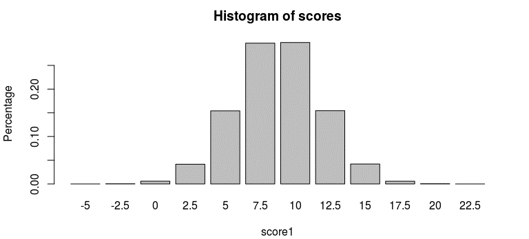
图 11-1
如果该集合不用了，就可以用 drop( ) 函数删除它：
m$drop( )
## [1] TRUE
因为这部分内容仅停留在介绍层面，MongoDB 的更多高级操作已超出了本书的范围。
如果你对 MongoDB 感兴趣，请浏览官方指南 https://docs.mongodb.com/manual/tutorial/。