机器学习——住房价格预测

一、选题背景

　　房价问题事关国计民生，已经成为全民关注的焦点议题之一。房地产更是我国最大的产业之一，对每个人对至关重要。本文主要对房价的合理性进行分析，根据测试集中各个房屋特征对销售价格的影响。并对此进行分析。估测了房价未来走势。同时进一步探讨使得房价合理的具体措施，根据分析结果，定量分析可能对经济发展产生的影响。

二、设计方案

　　本次机器学习设计具体方案，通过网上收集数据集，对数据集进行数据探索分析。然后对数据进行适当的数据清洗：异常值处理和缺失值处理。

　　1. 对数据做数据探索分析

　　2. 适当的数据清洗（异常值处理和缺失值处理）

　　3. 适当的特征工程

　　4. 用线性回归模型对房价进行预测

　　本次涉及的技术难点，本次作业用到线性回归模型（最小二乘、岭回归、Lasso）对房价进行预测，需要自己补充一下这方面的知识。#网上下载的测试集没有saleprice，只有将训练集ames_train分割成训练和测试集，随机采样20%的数据构建测试样本，其余作为训练样本。数据分析过程中对部分特征的分析不理解。解决方案是对看看别人的按理，学习一下其他人对数据的分析。

　　

数据集来源：kaggle：https://www.kaggle.com/competitions/plant-pathology-2021-fgvc8/data
kaggle：https://www.kaggle.com/competitions/plant-pathology-2020-fgvc7/data
参考案例：kaggle讨论区，csdn的kaggle房价预测项目https://blog.csdn.net/ttt123456uuu/article/details/119383848

三、实现步骤

获取数据集

 

 

 

(1）导入数据与工具包

import numpy as np # 矩阵操作
import pandas as pd # SQL数据处理
from sklearn.metrics import r2_score #评价回归预测模型的性能
import matplotlib.pyplot as plt #画图
import seaborn as sns
#忽略警告
import warnings
warnings.filterwarnings('ignore')
%matplotlib inline
#获取训练数据集
dpath = './data/'
ames_train = pd.read_csv(dpath+"Ames_House_train.csv")
#获取测试数据集
ames_test = pd.read_csv(dpath+"Ames_House_test.csv")
#观察训练集数据
ames_train.head()

 

 

 

 训练集总共有81个特征

#观察测试集数据
ames_test.head()

 

 

 

 80个特征，没有SalePrice，估计是要预测的集。最后可能只有从训练集抽一部分作为测试集

ames_train.info()

 

<class 'pandas.core.frame.DataFrame'>
RangeIndex: 1460 entries, 0 to 1459
Data columns (total 81 columns):
 #   Column         Non-Null Count  Dtype  
---  ------         --------------  -----  
 0   Id             1460 non-null   int64  
 1   MSSubClass     1460 non-null   int64  
 2   MSZoning       1460 non-null   object 
 3   LotFrontage    1201 non-null   float64
 4   LotArea        1460 non-null   int64  
 5   Street         1460 non-null   object 
 6   Alley          91 non-null     object 
 7   LotShape       1460 non-null   object 
 8   LandContour    1460 non-null   object 
 9   Utilities      1460 non-null   object 
 10  LotConfig      1460 non-null   object 
 11  LandSlope      1460 non-null   object 
 12  Neighborhood   1460 non-null   object 
 13  Condition1     1460 non-null   object 
 14  Condition2     1460 non-null   object 
 15  BldgType       1460 non-null   object 
 16  HouseStyle     1460 non-null   object 
 17  OverallQual    1460 non-null   int64  
 18  OverallCond    1460 non-null   int64  
 19  YearBuilt      1460 non-null   int64  
 20  YearRemodAdd   1460 non-null   int64  
 21  RoofStyle      1460 non-null   object 
 22  RoofMatl       1460 non-null   object 
 23  Exterior1st    1460 non-null   object 
 24  Exterior2nd    1460 non-null   object 
 25  MasVnrType     1452 non-null   object 
 26  MasVnrArea     1452 non-null   float64
 27  ExterQual      1460 non-null   object 
 28  ExterCond      1460 non-null   object 
 29  Foundation     1460 non-null   object 
 30  BsmtQual       1423 non-null   object 
 31  BsmtCond       1423 non-null   object 
 32  BsmtExposure   1422 non-null   object 
 33  BsmtFinType1   1423 non-null   object 
 34  BsmtFinSF1     1460 non-null   int64  
 35  BsmtFinType2   1422 non-null   object 
 36  BsmtFinSF2     1460 non-null   int64  
 37  BsmtUnfSF      1460 non-null   int64  
 38  TotalBsmtSF    1460 non-null   int64  
 39  Heating        1460 non-null   object 
 40  HeatingQC      1460 non-null   object 
 41  CentralAir     1460 non-null   object 
 42  Electrical     1459 non-null   object 
 43  1stFlrSF       1460 non-null   int64  
 44  2ndFlrSF       1460 non-null   int64  
 45  LowQualFinSF   1460 non-null   int64  
 46  GrLivArea      1460 non-null   int64  
 47  BsmtFullBath   1460 non-null   int64  
 48  BsmtHalfBath   1460 non-null   int64  
 49  FullBath       1460 non-null   int64  
 50  HalfBath       1460 non-null   int64  
 51  BedroomAbvGr   1460 non-null   int64  
 52  KitchenAbvGr   1460 non-null   int64  
 53  KitchenQual    1460 non-null   object 
 54  TotRmsAbvGrd   1460 non-null   int64  
 55  Functional     1460 non-null   object 
 56  Fireplaces     1460 non-null   int64  
 57  FireplaceQu    770 non-null    object 
 58  GarageType     1379 non-null   object 
 59  GarageYrBlt    1379 non-null   float64
 60  GarageFinish   1379 non-null   object 
 61  GarageCars     1460 non-null   int64  
 62  GarageArea     1460 non-null   int64  
 63  GarageQual     1379 non-null   object 
 64  GarageCond     1379 non-null   object 
 65  PavedDrive     1460 non-null   object 
 66  WoodDeckSF     1460 non-null   int64  
 67  OpenPorchSF    1460 non-null   int64  
 68  EnclosedPorch  1460 non-null   int64  
 69  3SsnPorch      1460 non-null   int64  
 70  ScreenPorch    1460 non-null   int64  
 71  PoolArea       1460 non-null   int64  
 72  PoolQC         7 non-null      object 
 73  Fence          281 non-null    object 
 74  MiscFeature    54 non-null     object 
 75  MiscVal        1460 non-null   int64  
 76  MoSold         1460 non-null   int64  
 77  YrSold         1460 non-null   int64  
 78  SaleType       1460 non-null   object 
 79  SaleCondition  1460 non-null   object 
 80  SalePrice      1460 non-null   int64  
dtypes: float64(3), int64(35), object(43)
memory usage: 924.0+ KB
object(43)型比较多，就是数据特征类别数据占了大多数吧

（2）数据探索

#分析SalePrice的情况
ames_train['SalePrice'].describe()

 

 

 

 1460个样本，最大值似乎有点高

#样本的SalePrice作正态分布曲线
sns.distplot(ames_train['SalePrice'])

 

 

 总体来看还算正常，集中分布在100000到250000这个区间，但是一直往右边延伸，说明最好的房子的价格是非常高的

#看看偏度（skewness）和峰度(peakedness)
print("Skewness: %f" % ames_train['SalePrice'].skew())
print("Kurtosis: %f" % ames_train['SalePrice'].kurt())

 

 

 (1)偏度：正态分布的偏度为0，两侧尾部长度对称。若以bs表示偏度。bs小于0称分布具有负偏离，也称左偏态，bs大于0称 分布具有正偏离，也称右偏态。

(2)峰度: 峰度为0表示该总体数据分布与正态分布的陡缓程度相同；峰度大于0表示该总体数据分布与正态分布相比较为陡 峭，为尖顶峰；峰度小于0表示该总体数据分布与正态分布相比较为平坦，为平顶峰。

因为小尾巴的存在，所以右偏，峰值也比较陡峭，saleprice比较集中

找几个感兴趣的特征来和SalePrice做散点图，首先看看数值型的特征:

#作散点图
#LotArea：土地的大小
var = 'LotArea'
data = pd.concat([ames_train['SalePrice'], ames_train[var]], axis=1)
data.plot.scatter(x=var, y='SalePrice', ylim=(0,800000));

 

 

 这里的土地应该是包括花园、操场空地的，大部分都比较小，估计是城区里的房子，LotArea比较大的可能是大农村，房价 高的房子一般土地都不小~

#作散点图
#GrLivArea：地上居住面积
var = 'GrLivArea'
data = pd.concat([ames_train['SalePrice'], ames_train[var]], axis=1)
data.plot.scatter(x=var, y='SalePrice', ylim=(0,800000));

 

 

 地上居住面积和价格，除了右下几个点以外，似乎呈线性分布,右下角的两个房子估计也是在农村，居住面积大，但是不值钱。

分析地下室面积:

#作散点图
#TotalBsmtSF：地下室总面积
var = 'TotalBsmtSF'
data = pd.concat([ames_train['SalePrice'], ames_train[var]], axis=1)
data.plot.scatter(x=var, y='SalePrice', ylim=(0,800000));

 

 

 除了极个别农村的房子，大部分还是呈线性分布，地下室越大价格越高，也注意到有些房子没有地下室。

分析类别型特征:

首先看看市区内的物理位置：

#Neighborhood:市内物理位置
var = 'Neighborhood'
data = pd.concat([ames_train['SalePrice'], ames_train[var]], axis=1)
f, ax = plt.subplots(figsize=(20, 8))
fig = sns.boxplot(x=var, y="SalePrice", data=data)
fig.axis(ymin=0, ymax=800000);

 

 

 看不出来什么明显趋势，大概只知道NoRideg、NridgHt和StoneBr这三地的房子要稍微贵一点吧 再来看看总体条件评级

#OverallQual:整体材质和完成品质
var = 'OverallQual'
data = pd.concat([ames_train['SalePrice'], ames_train[var]], axis=1)
f, ax = plt.subplots(figsize=(16, 8))
fig = sns.boxplot(x=var, y="SalePrice", data=data)
fig.axis(ymin=0, ymax=800000);

 

 

 既然是完成品质，肯定等级高的就越贵，所以这个趋势还是正常的

#OverallCond:总体条件评级
var = 'OverallCond'
data = pd.concat([ames_train['SalePrice'], ames_train[var]], axis=1)
f, ax = plt.subplots(figsize=(16, 8))
fig = sns.boxplot(x=var, y="SalePrice", data=data)
fig.axis(ymin=0, ymax=800000);

 

 

 总体评价等级，也基本能看出等级高价格贵，但是奇怪的是大部分价格高的房子集中再等级5。

#YearBuilt:最初建造日期
var = 'YearBuilt'
data = pd.concat([ames_train['SalePrice'], ames_train[var]], axis=1)
f, ax = plt.subplots(figsize=(20, 8))
fig = sns.boxplot(x=var, y="SalePrice", data=data)
fig.axis(ymin=0, ymax=800000);
plt.xticks(rotation=90);

 

 

 从建造日期来看，价格还算均匀分布，最老的房子和最新的房子价格较。 接下来构建一个相关性矩阵:

#correlation matrix热图，corr()计算相关性
corrmat = ames_train.corr()
f, ax = plt.subplots(figsize=(20, 12))
#vmax 能显示的最大值 vmin能显示的最小值
sns.heatmap(corrmat, vmax=0.9, square=True);

 

 

 通过热图，发现两组相关性比较高的属性

（1）地下室总面积（TotalBsmtSF）和第一层面积（1stFlrSF），难道国外第一层指的是地下室

（2）车库停放数量（GarageCars）和车库大小（GarageArea），车库大停车多，这个好理解。

选择10个与SalePrice最相关的属性作heatmap分析

k = 10 #相关属性数量
cols = corrmat.nlargest(k, 'SalePrice')['SalePrice'].index
cm = np.corrcoef(ames_train[cols].values.T)
sns.set(font_scale=1.25)
hm = sns.heatmap(cm, cbar=True, annot=True, square=True, fmt='.2f', annot_kws={'size': 10},
yticklabels=cols.values, xticklabels=cols.values)
plt.show()

 

 

 首先，GarageCars和GarageArea相关性达到了0.88，嗯车库越大停车越多，因此咱们去掉一个属性。考虑到GarageArea 和SalePrice的相关性比GarageCars和SalePrice的相关性低，那就把这个属性去掉吧。

GrLiveArea(地上居住面积)和TotRmsAbvGrd（地上房间总数）相关性也有0.83，房间多，居住面积就大，所以去掉 TotRmsAbvGrd。

TotalBsmtSF和1stFloor相关性0.82，同理去掉1stFloor

#去掉GarageArea（车库大小）、TotRmsAbvGrd（地上房间总数）、1stFlrSF（第一层面积）
ames_train = ames_train.drop('GarageArea', axis = 1)
ames_train = ames_train.drop('TotRmsAbvGrd', axis = 1)
ames_train = ames_train.drop('1stFlrSF', axis = 1)
ames_train.shape

(1460, 78)

降了三个维度

(3)数据缺失值处理

#数据缺失值处理
#首先看看哪些特征缺失的最多
total = ames_train.isnull().sum().sort_values(ascending=False)
percent = (ames_train.isnull().sum()/ames_train.isnull().count()).sort_values(ascending=False)
missing_data = pd.concat([total, percent], axis=1, keys=['Total', 'Percent'])
missing_data.head(20)

 

 

 来看看哪些特征缺失的比较多，首先是5个缺失最多特征：PoolQC、MiscFeature、Alley、Fence、FireplaceQu（有个百 分之80原则，若缺失80以上，就去掉该特征，但是这里缺失百分之50的也去掉了）

分别对应：游泳池质量、没被包含在其他类别的杂项功能 、所在巷通道的类型 、 围栏质量 、壁炉质量。

我想除了游泳池质量，很少有人会在乎后面四个特征吧，估计这也是信息缺失的原因。对于游泳池来讲，估计大多数房子都 没有游泳池，所以更不会有游泳池质量了，索性就先确定把这5个特征去掉吧。

#去掉PoolQC
ames_train = ames_train.drop(['PoolQC','MiscFeature','Alley','Fence','FireplaceQu'], axis = 1)

又去掉了5个特征。再来看看MasVnrArea（表明砌体面积）、MasVnrType（表明砌体类型）、Electrical（电气系统），注 意到这三个特征缺失值并不多，只有1个或者8个，所以直接把这几个含有缺失值的样本去掉。

#去掉Electrical有缺失值的样本
ames_train = ames_train.drop(ames_train.loc[ames_train['Electrical'].isnull()].index)
#去掉MasVnrArea有缺失值的样本
ames_train = ames_train.drop(ames_train.loc[ames_train['MasVnrArea'].isnull()].index)
#去掉MMasVnrType有缺失值的样本
ames_train = ames_train.drop(ames_train.loc[ames_train['MasVnrType'].isnull()].index)
ames_train.shape
(1451, 73)

经过以上处理以后，就只剩下缺失37个值到259个值的属性。

（1）如果直接删除这些属性，可能会造成大量有用的信息被浪费。

（2）如果删除包含缺失值的样本，就会导致样本数量下降259个，占了总样本的七分之一，更会丢失大量信息。

所以，综上所述，将剩余有缺失值的样本进行插值：

（1）对于数值型特征，考虑到平均数可能会被离群点拉高或者拉低，因此选择中位数来进行插值。

（2）对于类别型特征，直接将出现最多的类别填充到缺失值中另外，查资料还发现利用已有样本数据作回归，再将缺失值利用回归模型进行填充，在此就暂不作这样处理

#strategy ： ①若为mean时，用特征列的均值替换 ②若为median时，用特征列的中位数替换 ③若为most_frequent时，用特征
列的众数替换
#from sklearn.preprocessing import Imputer
#imputer=Imputer(missing_values='NaN', strategy='median', axis=0, verbose=0, copy=True)
#ames_train =imputer.fit_transform(ames_train)
#处理数值型特征，缺失值用中位数填补
ames_train=ames_train.fillna(ames_train.median())
#处理类别型特征，缺失值用该类别众数填补
#GarageType属性
ames_train['GarageType']=ames_train['GarageType'].fillna(ames_train['GarageType'].describe().top)
#GarageCond属性
ames_train['GarageCond']=ames_train['GarageCond'].fillna(ames_train['GarageCond'].describe().top)
#GarageFinish属性
ames_train['GarageFinish']=ames_train['GarageFinish'].fillna(ames_train['GarageFinish'].describe().t
op)
#GarageQual属性
ames_train['GarageQual']=ames_train['GarageQual'].fillna(ames_train['GarageQual'].describe().top)
#BsmtExposure属性
ames_train['BsmtExposure']=ames_train['BsmtExposure'].fillna(ames_train['BsmtExposure'].describe().t
op)
#BsmtFinType2属性
ames_train['BsmtFinType2']=ames_train['BsmtFinType2'].fillna(ames_train['BsmtFinType2'].describe().t
op)
#BsmtFinType1属性
ames_train['BsmtFinType1']=ames_train['BsmtFinType1'].fillna(ames_train['BsmtFinType1'].describe().t
op)
#BsmtCond属性
ames_train['BsmtCond']=ames_train['BsmtCond'].fillna(ames_train['BsmtCond'].describe().top)
#BsmtQual属性
ames_train['BsmtQual']=ames_train['BsmtQual'].fillna(ames_train['BsmtQual'].describe().top)
ames_train.shape
(1451, 73)
#观察下是否还有存在缺失值的特征
ames_train.isnull().sum().max()
0

显示为0，已经不存在缺失值了

ok,到这里缺失值就全部处理完了，接下来将类别标签进行编码

引入sklearn下的LabelEncoder包，用于对标签进行编码，编写一个类，用于对一个dataframe下的所有类别标签编码

from sklearn.pipeline import Pipeline
from sklearn.preprocessing import LabelEncoder
#定义一个类，可以将类别标签进行编码，e.g 假设四个标签，分别标为【1，2，3，4】
class MultiColumnLabelEncoder:
    def __init__(self,columns = None):
        self.columns = columns # array of column names to encode

    def fit(self,X,y=None):
        return self # not relevant here

    def transform(self,X):
        output = X.copy()
        if self.columns is not None:
            for col in self.columns:
                output[col] = LabelEncoder().fit_transform(output[col])
        else:
            for colname,col in output.iteritems():
                output[colname] = LabelEncoder().fit_transform(col)
        return output

    def fit_transform(self,X,y=None):
        return self.fit(X,y).transform(X)

#获取列类型为object的列，获取类别列
object_columns=[]
for col in ames_train.columns:
    if ames_train[col].dtypes=='object':
        object_columns.append(col)

#将类别特征string转化为数值型(0,1,2,3,4......)
ames_train=MultiColumnLabelEncoder(columns = object_columns).fit_transform(ames_train)

观察是否类别特征都已经转化成为数值

ames_train.head(20)

 

 

 (4)离群值处理

离群值(outlier)，也称逸出值，是指在数据中有一个或几个数值与其他数值相比差异较大。chanwennt准则规定，如果一个 数值偏离观测平均值的概率小于等于1/(2n)，则该数据应当舍弃（其中n为观察例数，概率可以很据数据的分布进行估计）。

　　　　　　　　----- ----摘自百度

首先来看看地面居住面积和房价的散点图，看是否存在离群

#地上居住面积
var = 'GrLivArea'
data = pd.concat([ames_train['SalePrice'], ames_train[var]], axis=1)
data.plot.scatter(x=var, y='SalePrice', ylim=(0,800000));

 

 

 可以看出数据主体依然呈线性关系，但是右下角的两个点比较碍眼，正如前面分析过的，可能是农村的房屋，所以面积大却 不值钱，由于偏离了主体，对线性回归模型会造成影响，所以就去掉右下角的两个样本。

右上方的两个点，看似离主群很远，但是实际上也在主群的方向上，所以不作处理

ames_train[(ames_train.GrLivArea>4500)]

 

 

 

#找到这两个离群点，删除他们
ames_train = ames_train.drop(ames_train[ames_train['Id'] == 1299].index)
ames_train = ames_train.drop(ames_train[ames_train['Id'] == 524].index)
ames_train.shape
(1449, 73)
#地下室总面积
var = 'TotalBsmtSF'
data = pd.concat([ames_train['SalePrice'], ames_train[var]], axis=1)
data.plot.scatter(x=var, y='SalePrice', ylim=(0,800000));

 

 

 右边的几个点虽然离主群较远，但总体来看依然呈线性分布的，所以也不作处理。

#低质量完成的面积
var = 'LowQualFinSF'
data = pd.concat([ames_train['SalePrice'], ames_train[var]], axis=1)
data.plot.scatter(x=var, y='SalePrice', ylim=(0,800000));

 

 

 可以看出大部分房屋，低质量完成的面积都是0。而最右边那个点，低质量完成面积那么大，反而价格还很高，我们把他提 取出来单独分析。

ames_train[(ames_train.LowQualFinSF>550)]

 

 

 

#取出该样本的总面积
lowQuaHouse=ames_train[ames_train.Id==186]
lowQuaHouse[['GrLivArea','TotalBsmtSF']]

 

 

 得出结论：低质量面积大概占总面积的8分之1，估计是大房子有部分没有装修完成，所以价格是合理的，这里就暂时不作处 理。

数据能符合统计学假设,作以下分析：

（1）正态性。（服从正态分布）

（2）方差齐性。（使独立变量在误差项相同）

（3）线性。

（4）无相关性错误。（特征之间正相关的误差造成负相关的误差）

首先是正态性

#histogram and normal probability plot
from scipy.stats import norm
from scipy import stats
sns.distplot(ames_train['SalePrice'], fit=norm);
fig = plt.figure()
res = stats.probplot(ames_train['SalePrice'], plot=plt)

 

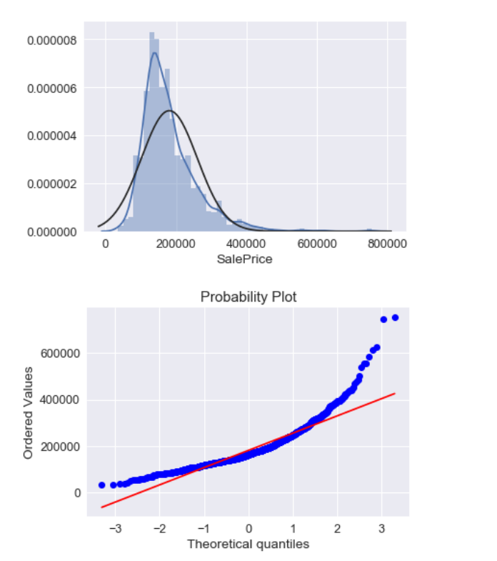
 SalePrice的分布不是标准正态型的，它呈现出来了峰度比较陡。

偏度也没有和对角线一致（不太明白这里的对角线是什么意思）

#使用log变换
ames_train['SalePrice'] = np.log(ames_train['SalePrice'])
sns.distplot(ames_train['SalePrice'], fit=norm);
fig = plt.figure()
res = stats.probplot(ames_train['SalePrice'], plot=plt)

 

 

 经过变换以后，峰度和偏度的问题都得到较好的修正。

接下来是GrLivArea（地上面积）特征：

sns.distplot(ames_train['GrLivArea'], fit=norm);
fig = plt.figure()
res = stats.probplot(ames_train['GrLivArea'], plot=plt)

 

 

 峰度比较符合正态分布，但是偏度稍微有点右偏。

#使用log变换
ames_train['GrLivArea'] = np.log(ames_train['GrLivArea'])
sns.distplot(ames_train['GrLivArea'], fit=norm);
fig = plt.figure()
res = stats.probplot(ames_train['GrLivArea'], plot=plt)

 

 

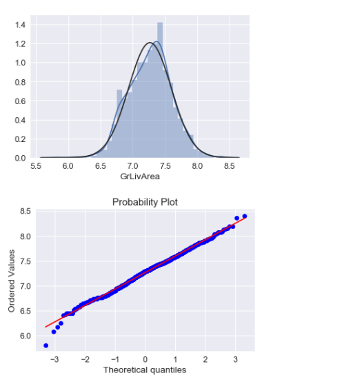
 log变换以后效果还不错。

#TotalBsmtSF正态分布特征
sns.distplot(ames_train['TotalBsmtSF'], fit=norm);
fig = plt.figure()
res = stats.probplot(ames_train['TotalBsmtSF'], plot=plt)

 

 

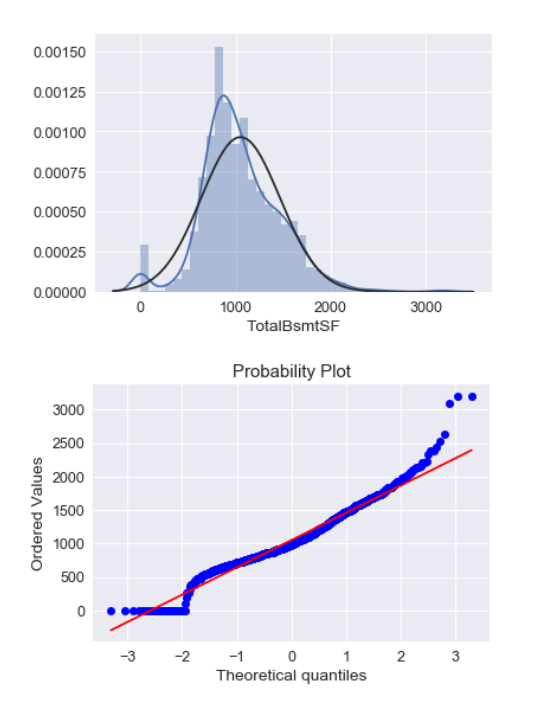
 问题出现了，有一些样本没有地下室，所以在TotalBsmtSF（地下室面积）这一项为0，为0那就不能使用log对数了啊 所以在这里对于地下室为0的样本就不作log处理，让它依然保持为0

#重新定义一项BsmtFlag，为0表示没有地下室，为1表示有地下室
ames_train['BsmtFlag'] = pd.Series(len(ames_train['TotalBsmtSF']), index=ames_train.index)
ames_train['BsmtFlag'] = 0
ames_train.loc[ames_train['TotalBsmtSF']>0,'BsmtFlag'] = 1
#log变换
ames_train.loc[ames_train['BsmtFlag']==1,'TotalBsmtSF'] = np.log(ames_train['TotalBsmtSF'])
#只列出了有地下室情况的正态分布特征
sns.distplot(ames_train[ames_train['TotalBsmtSF']>0]['TotalBsmtSF'], fit=norm);
fig = plt.figure()
res = stats.probplot(ames_train[ames_train['TotalBsmtSF']>0]['TotalBsmtSF'], plot=plt)

 

 

 转换后都样本的正态性都体现出来了 但是为什么在对角线上，总有一些点在首尾部分都偏移对角线很远呢？

#把新增的BsmtFlag列去掉
ames_train=ames_train.drop('BsmtFlag', axis = 1)
ames_train.shape
(1449, 73)

方差齐性探索

解决了正态性问题，再来看看方差齐性

plt.scatter(ames_train['GrLivArea'], ames_train['SalePrice']);

 

 

 

plt.scatter(ames_train[ames_train['TotalBsmtSF']>0]['TotalBsmtSF'],
ames_train[ames_train['TotalBsmtSF']>0]['SalePrice']);

 

 

 在作log转换处理前，样本分布呈圆锥型（可以查看前面特征与SalePrice的关系散点图），在低值处收于一小区域，在高值 处具有发散的特点。作log转换处理后，高值处的离散程度得到降低，两个样本的均值偏离程度变小，使其分布更集中，更符合 线性分布。

总结一下：

（1）log变换可以使数据分布更靠近正态分布模型；

（2）log变化可以使数据分布呈现方差齐性

(5）特征工程

#网上下载的测试集没有saleprice，只有将训练集ames_train分割成训练和测试集。。。。
#另外当数据较少时，可以考虑使用交叉验证，来扩充数据大小
# 从原始数据中分离输入特征x和输出y
y = ames_train['SalePrice'].values
#还要去掉编号ID
X = ames_train.drop(['SalePrice','Id'], axis = 1)
#将数据分割训练数据与测试数据
from sklearn.model_selection import train_test_split
# 随机采样20%的数据构建测试样本，其余作为训练样本
X_train, X_test, y_train, y_test = train_test_split(X, y, random_state=33, test_size=0.2)

查阅了一下标准化和归一化的区别:

(1)归一化特点 对不同特征维度的伸缩变换的目的是使各个特征维度对目标函数的影响权重是一致的，即使得那些扁平分布的数据伸缩变换 成类圆形。这也就改变了原始数据的一个分布。

好处： 1 提高迭代求解的收敛速度 2 提高迭代求解的精度

(2)标准化特点 对不同特征维度的伸缩变换的目的是使得不同度量之间的特征具有可比性。同时不改变原始数据的分布。

好处:

1 使得不同度量之间的特征具有可比性，对目标函数的影响体现在几何分布上，而不是数值上

2 不改变原始数据的分布

归一化会改变原始数据分布，似乎有些不妥。所以使用标准化吧

# 数据标准化
from sklearn.preprocessing import StandardScaler
# 分别初始化对特征和目标值的标准化器
ss_X = StandardScaler()
ss_y = StandardScaler()
# 分别对训练和测试数据的特征以及目标值进行标准化处理
X_train = ss_X.fit_transform(X_train)
X_test = ss_X.transform(X_test)
#对y做标准化不是必须
#对y标准化的好处是不同问题的w差异不太大，同时正则参数的范围也有限
y_train = ss_y.fit_transform(y_train.reshape(-1, 1))
y_test = ss_y.transform(y_test.reshape(-1, 1))

 

(6)确定模型类型

引入线性回归模型

columns = X.columns
# 线性回归
#class sklearn.linear_model.LinearRegression(fit_intercept=True, normalize=False, copy_X=True,
n_jobs=1)
from sklearn.linear_model import LinearRegression
# 使用默认配置初始化
lr = LinearRegression()
# 训练模型参数
lr.fit(X_train, y_train)
# 预测
y_test_pred_lr = lr.predict(X_test)
y_train_pred_lr = lr.predict(X_train)
# 看看各特征的权重系数，系数的绝对值大小可视为该特征的重要性
fs = pd.DataFrame({"columns":list(columns), "coef":list((lr.coef_.T))})
fs.sort_values(by=['coef'],ascending=False)

 

 

 影响比较大的特征：

（1）GrLivArea（地上居住面积）：房子越大越值钱，这个权值肯定最大的。

（2）BsmtFinSF1（ 第一类型完成面积）：虽然不太清楚第一类型是什么，但是跟面积有关，也算是越大越之前。

（3）OverallQual（整体材质和完成品质 ）：完成品质高的房屋当然值钱。

（4）BsmtUnfSF （未完成的地下室总面积）：没有装修的地下室更受欢迎，可能是人们喜欢自己布置地下室

（N）TotalBsmtSF （地下室总面积）： 这个竟然成了负值

# 使用r2_score评价模型在测试集和训练集上的性能，并输出评估结果
#测试集
print ('The r2 score of LinearRegression on test is')
print(r2_score(y_test, y_test_pred_lr))
#训练集
print ('The r2 score of LinearRegression on train is')
print(r2_score(y_train, y_train_pred_lr))
The r2 score of LinearRegression on test is
0.9217323743543604
The r2 score of LinearRegression on train is
0.9176913214680575

在测试集竟然比在训练集表现要好？感觉在划分测试集和训练集时有点问题，划分的训练集分布可能不具有普片性~~

 

#在训练集上观察预测残差的分布，看是否符合模型假设：噪声为0均值的高斯噪声
f, ax = plt.subplots(figsize=(7, 5))
f.tight_layout()
ax.hist(y_train - y_train_pred_lr,bins=40, label='Residuals Linear', color='b', alpha=.5);
ax.set_title("Histogram of Residuals")
ax.legend(loc='best');

 

 

 

 

 

 残差分布符合基本正态分布特征，有点右skew，左边的残差接近2，可能是噪声造成的影响。

#还可以观察预测值与真值的散点图
plt.figure(figsize=(4, 3))
plt.scatter(y_train, y_train_pred_lr)
plt.plot([-3, 3], [-3, 3], '--k') #数据已经标准化，3倍标准差即可
plt.axis('tight')
plt.xlabel('True price')
plt.ylabel('Predicted price')
plt.tight_layout()

 

 

 在两端的值稍微有点偏差，推测也是噪声引起的

引入随机梯度下降优化模型

随机梯度下降一次迭代只会计算一个维度的下降方向，而梯度下降会综合所有维度，找出下降最快的方向。所以在多维度情 况下，随机梯度下降会比梯度下降收敛速度更快，这样做的坏处就是失去了精度。

 

 

 

# 线性模型，随机梯度下降优化模型参数
# 随机梯度下降一般在大数据集上应用，其实本项目不适合用
from sklearn.linear_model import SGDRegressor
# 使用默认配置初始化线
sgdr = SGDRegressor(max_iter=1000)
# 训练：参数估计
sgdr.fit(X_train, y_train)
# 预测
sgdr_y_predict_train = sgdr.predict(X_train)
sgdr_y_predict_test = sgdr.predict(X_test)
# 看看各特征的权重系数，系数的绝对值大小可视为该特征的重要性
fs = pd.DataFrame({"columns":list(columns), "coef":list((sgdr.coef_.T))})
fs.sort_values(by=['coef'],ascending=False)
# sgdr.coef_

 

 

 

 

 

 

 

 

 TotalBsmtSF （地下室总面积）： 这个仍然是负值!!!看来买房的人们不太在意地下室情况。

# 使用SGDRegressor模型自带的评估模块(评价准则为r2_score)，并输出评估结果
print('The value of default measurement of SGDRegressor on test is ')
print(sgdr.score(X_test, y_test))
#训练集
print('The value of default measurement of SGDRegressor on train is')
print(sgdr.score(X_train, y_train))

#在训练集上观察预测残差的分布，看是否符合模型假设：噪声为0均值的高斯噪声
f, ax = plt.subplots(figsize=(7, 5))
f.tight_layout()
ax.hist(y_train - sgdr_y_predict_train.reshape(-1, 1),bins=40, label='Residuals Linear', color='r', alpha=.5);
ax.set_title("Histogram of Residuals")
ax.legend(loc='best');

 

 

 

 

 

 

残差分布符合基本正态分布特征，和线性回归分布模型类型，左边的残差接近2，可能是噪声造成的影响。

引入L2正则化的线性回归模型(岭回归)

#岭回归／L2正则
#class sklearn.linear_model.RidgeCV(alphas=(0.1, 1.0, 10.0), fit_intercept=True,
# normalize=False, scoring=None, cv=None, gcv_mode=None,
# store_cv_values=False)
from sklearn.linear_model import RidgeCV
#设置超参数（正则参数）范围
#alphas = [ 0.01, 0.1, 1, 10,100]
n_alphas = 20
alphas = np.logspace(-5,2,n_alphas)
#生成一个RidgeCV实例
ridge = RidgeCV(alphas=alphas, store_cv_values=True)
#模型训练
ridge.fit(X_train, y_train)
#预测
y_test_pred_ridge = ridge.predict(X_test)
y_train_pred_ridge = ridge.predict(X_train)
# 评估，使用r2_score评价模型在测试集和训练集上的性能
print ('The r2 score of RidgeCV on test is', r2_score(y_test, y_test_pred_ridge))
print ('The r2 score of RidgeCV on train is', r2_score(y_train, y_train_pred_ridge))

 

可视化

 

 

mse_mean = np.mean(ridge.cv_values_, axis = 0)
plt.plot(np.log10(alphas), mse_mean.reshape(len(alphas),1))
#这是为了标出最佳参数的位置，不是必须
plt.plot(np.log10(ridge.alpha_)*np.ones(3), [0.099, 0.1, 0.101])
plt.xlabel('log(alpha)')
plt.ylabel('mse')
plt.show()
print ('alpha is:', ridge.alpha_)

 

 

 

 

 

 使L2正则的目标函数最小的alpha取值为18.32980710832434

# 看看各特征的权重系数，系数的绝对值大小可视为该特征的重要性
fs = pd.DataFrame({"columns":list(columns), "coef_lr":list((lr.coef_.T)),
"coef_ridge":list((ridge.coef_.T))})
fs.sort_values(by=['coef_lr'],ascending=False)

 

 

 

总结一下：

（1）对比线性回归和L2正则的线性回归来看，在权值分布上，差别并不是太大

（2）L2正则会使权值趋于非常小，但是在这个例子上似乎没有体现出来

（3）带L2正则的线性回归在测试集上略好于一般线性回归，但是在训练集上又略差与一般线性回归，这体现了L2正则消除 过拟合的特点，即降低训练集表现，提高测试集表现

引入L1正则化的线性回归模型(Lasso)

#### Lasso／L1正则
# class sklearn.linear_model.LassoCV(eps=0.001, n_alphas=100, alphas=None, fit_intercept=True,
#                                    normalize=False, precompute=’auto’, max_iter=1000,
#                                    tol=0.0001, copy_X=True, cv=None, verbose=False, n_jobs=1,
#                                    positive=False, random_state=None, selection=’cyclic’)
from sklearn.linear_model import LassoCV

#设置超参数搜索范围
#alphas = [ 0.01, 0.1, 1, 10,100]
n_alphas = 20
alphas = np.logspace(-5,2,n_alphas)
#生成一个LassoCV实例
lasso = LassoCV(alphas=alphas)
#lasso = LassoCV()

#训练（内含CV）
lasso.fit(X_train, y_train)

#测试
y_test_pred_lasso = lasso.predict(X_test)
y_train_pred_lasso = lasso.predict(X_train)


# 评估，使用r2_score评价模型在测试集和训练集上的性能
print ('The r2 score of LassoCV on test is', r2_score(y_test, y_test_pred_lasso))
print ('The r2 score of LassoCV on train is', r2_score(y_train, y_train_pred_lasso))

 

 

 

可视化

 

mses = np.mean(lasso.mse_path_, axis = 1)
plt.plot(np.log10(lasso.alphas_), mses)
#plt.plot(np.log10(lasso.alphas_)*np.ones(3),[0.1, 0.2, 0.3])
plt.xlabel('log(alpha)')
plt.ylabel('mse')
plt.show()
print ('alpha is:', lasso.alpha_)

 

 

 

alpha is: 0.008858667904100823
使L1正则的目标函数最小的alpha取值为0.008858667904100823

# 看看各特征的权重系数，系数的绝对值大小可视为该特征的重要性
fs = pd.DataFrame({"columns":list(columns), "coef_lr":list((lr.coef_.T)),
"coef_ridge":list((ridge.coef_.T)), "coef_lasso":list((lasso.coef_.T))})
fs.sort_values(by=['coef_lr'],ascending=False)

 

 

 

 

总结一下：

（1）对比线性回归和L2正则的线性回归来看，L1正则线性回归在权值分布上，和前两者有相对较大的区别

（2）L1正则产生了稀疏性，许多权值都为0，据说这样的训练速度相对较快（没有亲测过）。

（3）带L1正则的线性回归在整体表现上要比L2正则和一般线性回归都要差一点。

四、总结

整个作业算是对线性回归有了总体的认识，从最开始的数据的分析、清洗，到最后模型的比较都需要仔细的研究。

（1）知道了正态分布的峰度和偏度，并对其有了初步的理解。

（2）了解了相关性矩阵，可以据此将相关性较大的属性去掉，降低特征工程的维度

（3）掌握了数据缺失值的方法，比如较多缺失值的可以直接删除该属性，较少缺失值的可以删除该样本，其余的进行插值 处理，可以用众数、中位数、平均数待敌缺失值，还有线性分析插值以及拉格朗日插值方法需要去探索学习。

（4）掌握了类别特征的编码，将期类别属性转化为数值属性。

（5）log变换使属性呈正态分布以及方差齐性的特点，有助于数据处理。

（6）了解了标准化和归一化的优缺点。

（7）对线性回归模型以及正则化防止过拟合有了一定的认识

结论

（1）GrLivArea（地上居住面积）：房子越大越值钱，这个权值肯定最大的。

（2）BsmtFinSF1（ 第一类型完成面积）：虽然不太清楚第一类型是什么，但是跟面积有关，也算是越大越之前。

（3）OverallQual（整体材质和完成品质 ）：完成品质高的房屋当然值钱。

（4）BsmtUnfSF （未完成的地下室总面积）：没有装修的地下室更受欢迎，可能是人们喜欢自己布置地下室

（N）TotalBsmtSF （地下室总面积）： 这个竟然成了负值。

通过线性回归模型得到了房屋销售价格中房屋各个特征的权重，以此了解了影响房屋销售价格的各种因素。可以凭此估测了房价未来走势。同时将来进一步探讨使得房价合理的具体措施。

以下附上完整代码：

import numpy as np  # 矩阵操作
import pandas as pd # SQL数据处理
from sklearn.metrics import r2_score  #评价回归预测模型的性能
import matplotlib.pyplot as plt   #画图
import seaborn as sns

#忽略警告
import warnings
warnings.filterwarnings('ignore')

#获取训练数据集
dpath = './data/'
ames_train = pd.read_csv(dpath+"Ames_House_train.csv")
#获取测试数据集
ames_test = pd.read_csv(dpath+"Ames_House_test.csv")

#观察训练集数据
ames_train.head()
#观察测试集数据
ames_test.head()

ames_train.info()
#分析SalePrice的情况
ames_train['SalePrice'].describe()
#样本的SalePrice作正态分布曲线
sns.distplot(ames_train['SalePrice']);

#看看偏度（skewness）和峰度(peakedness)
print("Skewness: %f" % ames_train['SalePrice'].skew())
print("Kurtosis: %f" % ames_train['SalePrice'].kurt())

#作散点图
#LotArea：土地的大小
var = 'LotArea'
data = pd.concat([ames_train['SalePrice'], ames_train[var]], axis=1)
data.plot.scatter(x=var, y='SalePrice', ylim=(0,800000));

#作散点图
#GrLivArea：地上居住面积
var = 'GrLivArea'
data = pd.concat([ames_train['SalePrice'], ames_train[var]], axis=1)
data.plot.scatter(x=var, y='SalePrice', ylim=(0,800000));

#作散点图
#TotalBsmtSF：地下室总面积
var = 'TotalBsmtSF'
data = pd.concat([ames_train['SalePrice'], ames_train[var]], axis=1)
data.plot.scatter(x=var, y='SalePrice', ylim=(0,800000));

#Neighborhood:市内物理位置
var = 'Neighborhood'
data = pd.concat([ames_train['SalePrice'], ames_train[var]], axis=1)
f, ax = plt.subplots(figsize=(20, 8))
fig = sns.boxplot(x=var, y="SalePrice", data=data)
fig.axis(ymin=0, ymax=800000);

#OverallQual:整体材质和完成品质
var = 'OverallQual'
data = pd.concat([ames_train['SalePrice'], ames_train[var]], axis=1)
f, ax = plt.subplots(figsize=(16, 8))
fig = sns.boxplot(x=var, y="SalePrice", data=data)
fig.axis(ymin=0, ymax=800000);

#OverallCond:总体条件评级
var = 'OverallCond'
data = pd.concat([ames_train['SalePrice'], ames_train[var]], axis=1)
f, ax = plt.subplots(figsize=(16, 8))
fig = sns.boxplot(x=var, y="SalePrice", data=data)
fig.axis(ymin=0, ymax=800000);

#YearBuilt:最初建造日期
var = 'YearBuilt'
data = pd.concat([ames_train['SalePrice'], ames_train[var]], axis=1)
f, ax = plt.subplots(figsize=(20, 8))
fig = sns.boxplot(x=var, y="SalePrice", data=data)
fig.axis(ymin=0, ymax=800000);
plt.xticks(rotation=90);

#correlation matrix热图，corr()计算相关性
corrmat = ames_train.corr()
f, ax = plt.subplots(figsize=(20, 12))
#vmax 能显示的最大值 vmin能显示的最小值
sns.heatmap(corrmat, vmax=0.9, square=True);

k = 10 #相关属性数量
cols = corrmat.nlargest(k, 'SalePrice')['SalePrice'].index
cm = np.corrcoef(ames_train[cols].values.T)
sns.set(font_scale=1.25)
hm = sns.heatmap(cm, cbar=True, annot=True, square=True, fmt='.2f', annot_kws={'size': 10}, yticklabels=cols.values, xticklabels=cols.values)
plt.show()

#去掉GarageArea（车库大小）、TotRmsAbvGrd（地上房间总数）、1stFlrSF（第一层面积）
ames_train = ames_train.drop('GarageArea', axis = 1)
ames_train = ames_train.drop('TotRmsAbvGrd', axis = 1)
ames_train = ames_train.drop('1stFlrSF', axis = 1)
ames_train.shape

#数据缺失值处理
#首先看看哪些特征缺失的最多
total = ames_train.isnull().sum().sort_values(ascending=False)
percent = (ames_train.isnull().sum()/ames_train.isnull().count()).sort_values(ascending=False)
missing_data = pd.concat([total, percent], axis=1, keys=['Total', 'Percent'])
missing_data.head(20)

#去掉PoolQC
ames_train = ames_train.drop(['PoolQC','MiscFeature','Alley','Fence','FireplaceQu'], axis = 1)

#去掉Electrical有缺失值的样本
ames_train = ames_train.drop(ames_train.loc[ames_train['Electrical'].isnull()].index)
#去掉MasVnrArea有缺失值的样本
ames_train = ames_train.drop(ames_train.loc[ames_train['MasVnrArea'].isnull()].index)
#去掉MMasVnrType有缺失值的样本
ames_train = ames_train.drop(ames_train.loc[ames_train['MasVnrType'].isnull()].index)

ames_train.shape

#strategy ：  ①若为mean时，用特征列的均值替换  ②若为median时，用特征列的中位数替换  ③若为most_frequent时，用特征列的众数替换

#处理数值型特征，缺失值用中位数填补
ames_train=ames_train.fillna(ames_train.median())

#处理类别型特征，缺失值用该类别众数填补
#GarageType属性
ames_train['GarageType']=ames_train['GarageType'].fillna(ames_train['GarageType'].describe().top)
#GarageCond属性
ames_train['GarageCond']=ames_train['GarageCond'].fillna(ames_train['GarageCond'].describe().top)
#GarageFinish属性
ames_train['GarageFinish']=ames_train['GarageFinish'].fillna(ames_train['GarageFinish'].describe().top)
#GarageQual属性
ames_train['GarageQual']=ames_train['GarageQual'].fillna(ames_train['GarageQual'].describe().top)
#BsmtExposure属性
ames_train['BsmtExposure']=ames_train['BsmtExposure'].fillna(ames_train['BsmtExposure'].describe().top)
#BsmtFinType2属性
ames_train['BsmtFinType2']=ames_train['BsmtFinType2'].fillna(ames_train['BsmtFinType2'].describe().top)
#BsmtFinType1属性
ames_train['BsmtFinType1']=ames_train['BsmtFinType1'].fillna(ames_train['BsmtFinType1'].describe().top)
#BsmtCond属性
ames_train['BsmtCond']=ames_train['BsmtCond'].fillna(ames_train['BsmtCond'].describe().top)
#BsmtQual属性
ames_train['BsmtQual']=ames_train['BsmtQual'].fillna(ames_train['BsmtQual'].describe().top)

ames_train.shape

#观察下是否还有存在缺失值的特征
ames_train.isnull().sum().max()

from sklearn.pipeline import Pipeline
from sklearn.preprocessing import LabelEncoder
#定义一个类，可以将类别标签进行编码，e.g 假设四个标签，分别标为【1，2，3，4】
class MultiColumnLabelEncoder:
    def __init__(self,columns = None):
        self.columns = columns # array of column names to encode

    def fit(self,X,y=None):
        return self # not relevant here

    def transform(self,X):
        output = X.copy()
        if self.columns is not None:
            for col in self.columns:
                output[col] = LabelEncoder().fit_transform(output[col])
        else:
            for colname,col in output.iteritems():
                output[colname] = LabelEncoder().fit_transform(col)
        return output

    def fit_transform(self,X,y=None):
        return self.fit(X,y).transform(X)

#获取列类型为object的列，获取类别列
object_columns=[]
for col in ames_train.columns:
    if ames_train[col].dtypes=='object':
        object_columns.append(col)

#将类别特征string转化为数值型(0,1,2,3,4......)
ames_train=MultiColumnLabelEncoder(columns = object_columns).fit_transform(ames_train)

ames_train.head(20)

#地上居住面积
var = 'GrLivArea'
data = pd.concat([ames_train['SalePrice'], ames_train[var]], axis=1)
data.plot.scatter(x=var, y='SalePrice', ylim=(0,800000));

ames_train[(ames_train.GrLivArea>4500)]

#找到这两个离群点，删除他们
ames_train = ames_train.drop(ames_train[ames_train['Id'] == 1299].index)
ames_train = ames_train.drop(ames_train[ames_train['Id'] == 524].index)
ames_train.shape

#地下室总面积
var = 'TotalBsmtSF'
data = pd.concat([ames_train['SalePrice'], ames_train[var]], axis=1)
data.plot.scatter(x=var, y='SalePrice', ylim=(0,800000));

#低质量完成的面积
var = 'LowQualFinSF'
data = pd.concat([ames_train['SalePrice'], ames_train[var]], axis=1)
data.plot.scatter(x=var, y='SalePrice', ylim=(0,800000));

ames_train[(ames_train.LowQualFinSF>550)]

#取出该样本的总面积
lowQuaHouse=ames_train[ames_train.Id==186]
lowQuaHouse[['GrLivArea','TotalBsmtSF']]

#histogram and normal probability plot
from scipy.stats import norm
from scipy import stats
sns.distplot(ames_train['SalePrice'], fit=norm);
fig = plt.figure()
res = stats.probplot(ames_train['SalePrice'], plot=plt)

#使用log变换
ames_train['SalePrice'] = np.log(ames_train['SalePrice'])

sns.distplot(ames_train['SalePrice'], fit=norm);
fig = plt.figure()
res = stats.probplot(ames_train['SalePrice'], plot=plt)

sns.distplot(ames_train['GrLivArea'], fit=norm);
fig = plt.figure()
res = stats.probplot(ames_train['GrLivArea'], plot=plt)

#使用log变换
ames_train['GrLivArea'] = np.log(ames_train['GrLivArea'])

sns.distplot(ames_train['GrLivArea'], fit=norm);
fig = plt.figure()
res = stats.probplot(ames_train['GrLivArea'], plot=plt)

#TotalBsmtSF正态分布特征
sns.distplot(ames_train['TotalBsmtSF'], fit=norm);
fig = plt.figure()
res = stats.probplot(ames_train['TotalBsmtSF'], plot=plt)

#重新定义一项BsmtFlag，为0表示没有地下室，为1表示有地下室
ames_train['BsmtFlag'] = pd.Series(len(ames_train['TotalBsmtSF']), index=ames_train.index)
ames_train['BsmtFlag'] = 0
ames_train.loc[ames_train['TotalBsmtSF']>0,'BsmtFlag'] = 1
#log变换
ames_train.loc[ames_train['BsmtFlag']==1,'TotalBsmtSF'] = np.log(ames_train['TotalBsmtSF'])

#只列出了有地下室情况的正态分布特征
sns.distplot(ames_train[ames_train['TotalBsmtSF']>0]['TotalBsmtSF'], fit=norm);
fig = plt.figure()
res = stats.probplot(ames_train[ames_train['TotalBsmtSF']>0]['TotalBsmtSF'], plot=plt)

#把新增的BsmtFlag列去掉
ames_train=ames_train.drop('BsmtFlag', axis = 1)
ames_train.shape

plt.scatter(ames_train['GrLivArea'], ames_train['SalePrice']);

plt.scatter(ames_train[ames_train['TotalBsmtSF']>0]['TotalBsmtSF'], ames_train[ames_train['TotalBsmtSF']>0]['SalePrice']);

#网上下载的测试集没有saleprice，只有将训练集ames_train分割成训练和测试集。。。。
#另外当数据较少时，可以考虑使用交叉验证，来扩充数据大小

# 从原始数据中分离输入特征x和输出y
y = ames_train['SalePrice'].values

#还要去掉编号ID
X = ames_train.drop(['SalePrice','Id'], axis = 1)

#将数据分割训练数据与测试数据
from sklearn.model_selection import train_test_split

# 随机采样20%的数据构建测试样本，其余作为训练样本
X_train, X_test, y_train, y_test = train_test_split(X, y, random_state=33, test_size=0.2)

# 数据标准化
from sklearn.preprocessing import StandardScaler

# 分别初始化对特征和目标值的标准化器
ss_X = StandardScaler()
ss_y = StandardScaler()

# 分别对训练和测试数据的特征以及目标值进行标准化处理
X_train = ss_X.fit_transform(X_train)
X_test = ss_X.transform(X_test)

#对y做标准化不是必须
#对y标准化的好处是不同问题的w差异不太大，同时正则参数的范围也有限
y_train = ss_y.fit_transform(y_train.reshape(-1, 1))
y_test = ss_y.transform(y_test.reshape(-1, 1))

columns = X.columns
# 线性回归
#class sklearn.linear_model.LinearRegression(fit_intercept=True, normalize=False, copy_X=True, n_jobs=1)
from sklearn.linear_model import LinearRegression

# 使用默认配置初始化
lr = LinearRegression()

# 训练模型参数
lr.fit(X_train, y_train)

# 预测
y_test_pred_lr = lr.predict(X_test)
y_train_pred_lr = lr.predict(X_train)


# 看看各特征的权重系数，系数的绝对值大小可视为该特征的重要性
fs = pd.DataFrame({"columns":list(columns), "coef":list((lr.coef_.T))})
fs.sort_values(by=['coef'],ascending=False)

# 使用r2_score评价模型在测试集和训练集上的性能，并输出评估结果
#测试集
print ('The r2 score of LinearRegression on test is')
print(r2_score(y_test, y_test_pred_lr))
#训练集
print ('The r2 score of LinearRegression on train is')
print(r2_score(y_train, y_train_pred_lr))

#在训练集上观察预测残差的分布，看是否符合模型假设：噪声为0均值的高斯噪声
f, ax = plt.subplots(figsize=(7, 5))
f.tight_layout()
ax.hist(y_train - y_train_pred_lr,bins=40, label='Residuals Linear', color='b', alpha=.5);
ax.set_title("Histogram of Residuals")
ax.legend(loc='best');

#还可以观察预测值与真值的散点图
plt.figure(figsize=(4, 3))
plt.scatter(y_train, y_train_pred_lr)
plt.plot([-3, 3], [-3, 3], '--k')   #数据已经标准化，3倍标准差即可
plt.axis('tight')
plt.xlabel('True price')
plt.ylabel('Predicted price')
plt.tight_layout()

# 线性模型，随机梯度下降优化模型参数
# 随机梯度下降一般在大数据集上应用，其实本项目不适合用
from sklearn.linear_model import SGDRegressor

# 使用默认配置初始化线
sgdr = SGDRegressor(max_iter=1000)

# 训练：参数估计
sgdr.fit(X_train, y_train)

# 预测
sgdr_y_predict_train = sgdr.predict(X_train)
sgdr_y_predict_test = sgdr.predict(X_test)

# 看看各特征的权重系数，系数的绝对值大小可视为该特征的重要性
fs = pd.DataFrame({"columns":list(columns), "coef":list((sgdr.coef_.T))})
fs.sort_values(by=['coef'],ascending=False)
# sgdr.coef_

# 使用SGDRegressor模型自带的评估模块(评价准则为r2_score)，并输出评估结果
print('The value of default measurement of SGDRegressor on test is ')
print(sgdr.score(X_test, y_test))
#训练集
print('The value of default measurement of SGDRegressor on train is')
print(sgdr.score(X_train, y_train))

#在训练集上观察预测残差的分布，看是否符合模型假设：噪声为0均值的高斯噪声
f, ax = plt.subplots(figsize=(7, 5))
f.tight_layout()
ax.hist(y_train - sgdr_y_predict_train.reshape(-1, 1),bins=40, label='Residuals Linear', color='r', alpha=.5);
ax.set_title("Histogram of Residuals")
ax.legend(loc='best');

#岭回归／L2正则
#class sklearn.linear_model.RidgeCV(alphas=(0.1, 1.0, 10.0), fit_intercept=True,
#                                  normalize=False, scoring=None, cv=None, gcv_mode=None,
#                                  store_cv_values=False)
from sklearn.linear_model import  RidgeCV

#设置超参数（正则参数）范围
#alphas = [ 0.01, 0.1, 1, 10,100]

n_alphas = 20
alphas = np.logspace(-5,2,n_alphas)

#生成一个RidgeCV实例
ridge = RidgeCV(alphas=alphas, store_cv_values=True)

#模型训练
ridge.fit(X_train, y_train)

#预测
y_test_pred_ridge = ridge.predict(X_test)
y_train_pred_ridge = ridge.predict(X_train)


# 评估，使用r2_score评价模型在测试集和训练集上的性能
print ('The r2 score of RidgeCV on test is', r2_score(y_test, y_test_pred_ridge))
print ('The r2 score of RidgeCV on train is', r2_score(y_train, y_train_pred_ridge))

mse_mean = np.mean(ridge.cv_values_, axis = 0)
plt.plot(np.log10(alphas), mse_mean.reshape(len(alphas),1))

#这是为了标出最佳参数的位置，不是必须
plt.plot(np.log10(ridge.alpha_)*np.ones(3), [0.099, 0.1, 0.101])

plt.xlabel('log(alpha)')
plt.ylabel('mse')
plt.show()

print ('alpha is:', ridge.alpha_)

# 看看各特征的权重系数，系数的绝对值大小可视为该特征的重要性
fs = pd.DataFrame({"columns":list(columns), "coef_lr":list((lr.coef_.T)), "coef_ridge":list((ridge.coef_.T))})
fs.sort_values(by=['coef_lr'],ascending=False)

#### Lasso／L1正则
# class sklearn.linear_model.LassoCV(eps=0.001, n_alphas=100, alphas=None, fit_intercept=True,
#                                    normalize=False, precompute=’auto’, max_iter=1000,
#                                    tol=0.0001, copy_X=True, cv=None, verbose=False, n_jobs=1,
#                                    positive=False, random_state=None, selection=’cyclic’)
from sklearn.linear_model import LassoCV

#设置超参数搜索范围
#alphas = [ 0.01, 0.1, 1, 10,100]
n_alphas = 20
alphas = np.logspace(-5,2,n_alphas)
#生成一个LassoCV实例
lasso = LassoCV(alphas=alphas)
#lasso = LassoCV()

#训练（内含CV）
lasso.fit(X_train, y_train)

#测试
y_test_pred_lasso = lasso.predict(X_test)
y_train_pred_lasso = lasso.predict(X_train)


# 评估，使用r2_score评价模型在测试集和训练集上的性能
print ('The r2 score of LassoCV on test is', r2_score(y_test, y_test_pred_lasso))
print ('The r2 score of LassoCV on train is', r2_score(y_train, y_train_pred_lasso))

mses = np.mean(lasso.mse_path_, axis=1)
plt.plot(np.log10(lasso.alphas_), mses)

# plt.plot(np.log10(lasso.alphas_)*np.ones(3),[0.1, 0.2, 0.3])
plt.xlabel('log(alpha)')
plt.ylabel('mse')
plt.show()

print('alpha is:', lasso.alpha_)

# 看看各特征的权重系数，系数的绝对值大小可视为该特征的重要性
fs = pd.DataFrame({"columns":list(columns), "coef_lr":list((lr.coef_.T)), "coef_ridge":list((ridge.coef_.T)), "coef_lasso":list((lasso.coef_.T))})
fs.sort_values(by=['coef_lr'],ascending=False)