
萤火虫算法
1. 萤火虫优化算法背景
受萤火虫发光强度的启发,2008年,英国剑桥大学学者Xin-She Yang提出萤火虫算法(Firefly Algorithm, FA)。自然界中,萤火虫可以发出短促、有节奏的闪光。通常这种闪光仅在一定范围内可见。萤火虫通过闪光可以吸引异性和猎取食物。为了使算法更加简单,该算法只考虑了萤火虫强度的变化和吸引力这两个因素。
2. 萤火虫优化算法理想化数学模型
依照萤火虫发光的特性,给出以下理想化规则:
(1) 萤火虫不分雌雄,每个萤火虫都会被比它发光更亮的萤火虫吸引;
(2) 吸引力与发光强度成正比;
(3) 萤火虫的亮度由目标函数值决定。
3. 萤火虫优化算法的更新过程
3.1 绝对亮度的定义
为了表示萤火虫的亮度随距离的变化,定义如下绝对亮度:
萤火虫绝对亮度为距离时的亮度,记为.
注意:为了降低算法的复杂度,假定萤火虫的绝对亮度与的目标函数值相等。
3.2 相对亮度的定义
为了表示萤火虫对萤火虫的吸引大小,定义如下相对亮度:
萤火虫在萤火虫位置的光强度,记为
其中,为光吸收系数,为萤火虫到萤火虫的距离.
3.3 吸引力的定义
假设萤火虫对萤火虫的吸引力和萤火虫对萤火虫的相对亮度成比例,所以萤火虫对萤火虫的吸引力可表示为:
其中,为最大吸引力,当距离时,吸引力最大。通常,.
3.4 萤火虫位置更新公式
萤火虫吸引着萤火虫,因此萤火虫的位置更新公式:
其中,为算法的迭代次数;、分别为萤火虫和萤火虫所处的空间位置;, 是高斯分布得到的随机向量。
第一版本:
% =========================================================================
% Coder: Lee WenTsao
% Time: 2022-05-14
% Email: liwenchao36@163.com
% Reference: Xin-She Yang, Nature-Inspired Metaheuristic Algorithms,
% Luniver Press, First Edition.
% =========================================================================
%% 清理运行环境
clc
clear
close all
%% 问题定义
option = 2; % 选择优化函数
dimension = 2; % 维数
[fobj, bound] = Optimizer(option);
lb = bound(1); % 下界
ub = bound(2); % 上界
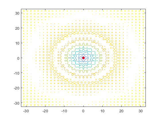
%% 绘制云图
figure(1)
x = linspace(lb, ub, 101);
y = linspace(lb, ub, 101);
z = zeros(101);
for i=1:length(x)
for j=1:length(y)
z(i,j) = fobj([x(i), y(j)]);
end
end
contour(x,y,z); % 函数云图显示
hold on;
%% 萤火虫参数设置
num_pop = 30; % 初始种群数目
Max_gen = 1000; % 最大迭代次数
beta_0 = 1.0; % 最大吸引力
gamma = 0.1; % 光强吸收系数
alpha = 1.0; % 步长因子
theta = 0.97; % alpha衰减因子
%% 初始化种群
Sol = zeros(num_pop, dimension);
I = zeros(num_pop, 1);
for i=1:num_pop
Sol(i,:) = lb + (ub - lb)*rand(1,dimension); % 初始化种群
I(i) = fobj(Sol(i,:)); % 适应度
end
[fmin, id] = min(I);
best_scores = [fmin];
%% 动态表示
points = scatter(Sol(:,1),Sol(:,2),"ro","filled");
xlim([lb,ub]);
ylim([lb,ub]);
drawnow;
%% 仿真
for iter=1:Max_gen
alpha = alpha*theta;
scale = abs((ub -lb)*ones(1, dimension)); % 优化问题的尺度
for i=1:num_pop
for j=1:num_pop
if I(i)>I(j)
% 计算萤火虫i和萤火虫j之间的距离
r = sqrt(sum((Sol(i,:) - Sol(j,:)).^2));
% 计算萤火虫之间的吸引力
beta = beta_0*exp(-gamma*r.^2);
% 搜索精度
steps = alpha.*(rand(1,dimension) - 0.5).*scale;
% 更新萤火虫的位置
S = Sol(i,:) + beta*(Sol(j,:) - Sol(i,:)) + steps;
% 萤火虫越界处理
Tp = S>ub;
Tm = S<lb;
S = S.*(~(Tp+Tm)) + ub.*Tp + lb.*Tm;
% 适应度值
new_fun = fobj(S);
% 进化机制
if new_fun<I(i)
Sol(i,:) = S;
I(i) = new_fun;
end
% 更新最优
if I(i)<fmin
fmin = I(i);
id = i;
end
end
end
end
best_scores = [best_scores,fmin];
reset(points);
points = scatter(Sol(:,1), Sol(:,2), 'ro','filled');
pause(0.1)
%% 输出
if ~mod(iter,50)
disp(['迭代次数:' num2str(iter) '|| 最优值:' num2str(fmin)]);
end
end
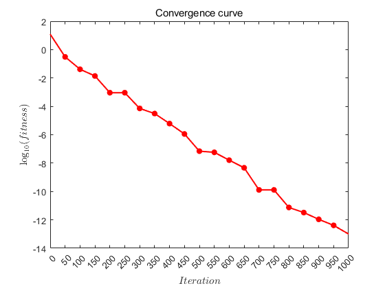
%% 收敛曲线可视化
figure(2)
xx = 1:50:1001;
xxx = 0:50:1000;
plot(xxx,log10(best_scores(xx)),'r','LineWidth',1.5);
hold on;
sz = 40;
scatter(xxx(2:end-1),log10(best_scores(xx(2:end-1))),sz,'ro','filled');
xlabel('$$Iteration$$','Interpreter','latex');
ylabel('$$\log_{10} (fitness)$$','Interpreter','latex');
title('Convergence curve')
xticks(0:50:1000);
杨老师原始版本:
% ---------------------------------------------------------------------- %
% The Firefly Algorithm (FA) for unconstrained function optimization     %
% by Xin-She Yang (Cambridge University) @2008-2009                      %
% Programming dates: 2008-2009, then revised and updated in Oct 2010     %
% ---------------------------------------------------------------------- %

% References -- citation details: -------------------------------------- %
% (1) Xin-She Yang, Nature-Inspired Metaheuristic Algorithms,            %
%     Luniver Press, First Edition, (2008).                              %
% (2) Xin-She Yang, Firefly Algorithm, Stochastic Test Functions and     %
%     Design Optimisation, Int. Journal of Bio-Inspired Computation,     %
%     vol. 2, no. 2, 78-84 (2010).                                       %
% ---------------------------------------------------------------------- %

% -------- Start the Firefly Algorithm (FA) main loop ------------------ %
function fa_ndim_new
n=20;                   % Population size (number of fireflies)
alpha=1.0;              % Randomness strength 0--1 (highly random)
beta0=1.0;              % Attractiveness constant
gamma=0.01;             % Absorption coefficient
theta=0.97;             % Randomness reduction factor theta=10^(-5/tMax)
d=10;                   % Number of dimensions
tMax=500;               % Maximum number of iterations
Lb=-10*ones(1,d);       % Lower bounds/limits
Ub=10*ones(1,d);        % Upper bounds/limits
% Generating the initial locations of n fireflies
for i=1:n,
   ns(i,:)=Lb+(Ub-Lb).*rand(1,d);         % Randomization
   Lightn(i)=cost(ns(i,:));               % Evaluate objectives
end

%%%%%%%%%%%%%%%%% Start the iterations (main loop) %%%%%%%%%%%%%%%%%%%%%%%
for k=1:tMax,
 alpha=alpha*theta;     % Reduce alpha by a factor theta
 scale=abs(Ub-Lb);      % Scale of the optimization problem
% Two loops over all the n fireflies
for i=1:n,
    for j=1:n,
      % Evaluate the objective values of current solutions
      Lightn(i)=cost(ns(i,:));           % Call the objective
      % Update moves
      if Lightn(i)>=Lightn(j),           % Brighter/more attractive
         r=sqrt(sum((ns(i,:)-ns(j,:)).^2));
         beta=beta0*exp(-gamma*r.^2);    % Attractiveness
         steps=alpha.*(rand(1,d)-0.5).*scale;
      % The FA equation for updating position vectors
         ns(i,:)=ns(i,:)+beta*(ns(j,:)-ns(i,:))+steps;
      end
   end % end for j
end % end for i

% Check if the new solutions/locations are within limits/bounds
ns=findlimits(n,ns,Lb,Ub);
%% Rank fireflies by their light intensity/objectives
[Lightn,Index]=sort(Lightn);
nsol_tmp=ns;
for i=1:n,
 ns(i,:)=nsol_tmp(Index(i),:);
end
%% Find the current best solution and display outputs
fbest=Lightn(1), nbest=ns(1,:)
end % End of the main FA loop (up to tMax)

% Make sure that new fireflies are within the bounds/limits
function [ns]=findlimits(n,ns,Lb,Ub)
for i=1:n,
  nsol_tmp=ns(i,:);
  % Apply the lower bound
  I=nsol_tmp<Lb;  nsol_tmp(I)=Lb(I);
  % Apply the upper bounds
  J=nsol_tmp>Ub;  nsol_tmp(J)=Ub(J);
  % Update this new move
  ns(i,:)=nsol_tmp;
end

%% Define the objective function or cost function
function z=cost(x)
% The modified sphere function: z=sum_{i=1}^D (x_i-1)^2
z=sum((x-1).^2); % The global minimum fmin=0 at (1,1,...,1)
% -----------------------------------------------------------------------%


【推荐】国内首个AI IDE,深度理解中文开发场景,立即下载体验Trae
【推荐】编程新体验,更懂你的AI,立即体验豆包MarsCode编程助手
【推荐】抖音旗下AI助手豆包,你的智能百科全书,全免费不限次数
【推荐】轻量又高性能的 SSH 工具 IShell:AI 加持,快人一步
· go语言实现终端里的倒计时
· 如何编写易于单元测试的代码
· 10年+ .NET Coder 心语,封装的思维:从隐藏、稳定开始理解其本质意义
· .NET Core 中如何实现缓存的预热?
· 从 HTTP 原因短语缺失研究 HTTP/2 和 HTTP/3 的设计差异
· 周边上新:园子的第一款马克杯温暖上架
· 分享 3 个 .NET 开源的文件压缩处理库,助力快速实现文件压缩解压功能!
· Ollama——大语言模型本地部署的极速利器
· DeepSeek如何颠覆传统软件测试?测试工程师会被淘汰吗?
· 使用C#创建一个MCP客户端