这篇文章相比于Segmentation-based deep- ˇ learning approach for surface-defect detection.这篇文章,首先他们都是一个作者写的,其次网络的架构也是非常接近的
为了保证小细节被保留下来,这里使用的是max-pool2x2,而不是使用stride=2的卷积,这里使用了3次的max-pool2x2, 用来构成分割的主体网络,从图中可以看出,Segmentation结果相比于原始图小了8倍,因此这里使用的分割标签low-level resolution,粗略的标签而不是精细的标签,因为作者认为相比于像素集的损失,判断是否有缺陷的分类结果更为重要。
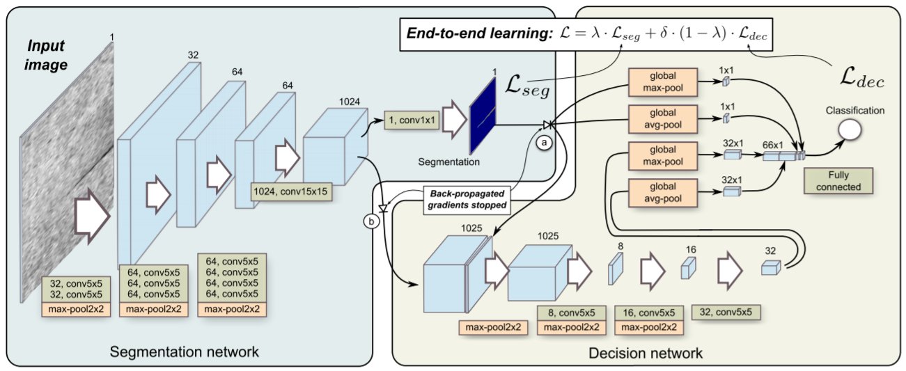
这里讲一下文章中所提到的四个关键优化点
1. Dynamically balanced loss
To implement end-to-end learning, we combine both losses, the segmentation loss and the classification loss, into a single unified loss, allowing for a simultaneous learning. New combined loss is defined as:
为了使用端到端的学习,我们融合了两种Loss, 分割loss和分类的loss,融合为一种简单统一loss,允许进行共同学习。新的loss如下:

where Lseg and Lcls represent segmentation and classification losses, respectively, δ is an additional classification loss weight that prevents the classification loss from dominating the total loss, while λ is a mixing factor that balances the contribution of each network in the final loss. Note that λ, and δ do not replace the learning rate η in SGD, but complement it. They adequately control the learning process, as losses can be in different scales. The segmentation loss is averaged over all the pixels, and more importantly, only a handful of pixels are anomalous, resulting in a relatively small values compared to the classification loss, therefore we normally use smaller δ values to prevent the classification loss from dominating the total loss.
这里Lseg和Lcls表示分割和分类的loss,各自的,δ是一个额外的分类损失权重这可以防止分类的loss占据总的Loss,λ是一个混合因子可以平衡不同网络在最终loss中的贡献。注意,λ, and δ不能替换SGD中的学习率,但是可以补充它。他们充分的控制着学习流程,作为在不同尺寸上的损失。这个Segmentation loss 是相对于所有像素的平均,更加重要,但是只有少了的像素值是目标,相比于分类损失这个数值就很小,因此我们使用一个更小的δ 数值来预防分类损失占据整个损失。
Learning the classification network before the segmentation network features are stable represents an additional challenge for the simultaneous learning. We address this by proposing to start learning only the segmentation network at the beginning and gradually progress towards learning only the classification part at the end. We formulate this by computing segmentation and classification mixing factors as a simple linear function:
在分割网络特征稳定前训练分类网络对于同时训练是另外一个挑战。我们处理这情况通过在开始的时候训练分割网络并且逐步学习在最后的时候训练分类网络。我们制定这个通过计算分割和分类的混合因子作为一个简单的线性函数

where n represents the index of the current epoch and total epoch represents the total number of training epochs. Without the gradual mixing of both losses, the learning would in some cases result in exploding gradients, thus making the model more difficult to use. We term the process of gradually including classification network and excluding segmentation network as a dynamically balanced loss. Additionally, using lower δ values further reduces the issue of learning on the noisy segmentation features early on, whereas using greater values has sometimes lead to the problem of exploding gradients.
这里n表示当前的epoch的索引值,total epoch 表示整个训练的epoch次数,没有两种损失函数的逐步混合,这个训练将会在一些情况下导致梯度爆炸,因此导致这个网络更加难以使用。我们把这个逐步包括分类网络且不包含分割网络的过程称为动态平衡损失函数,另外,进一步使用较低的δ values减少在早期学习到带有噪声的分割特征,然而使用较大的值有时候会导致梯度爆炸的问题
2.Gradient-flow adjustments
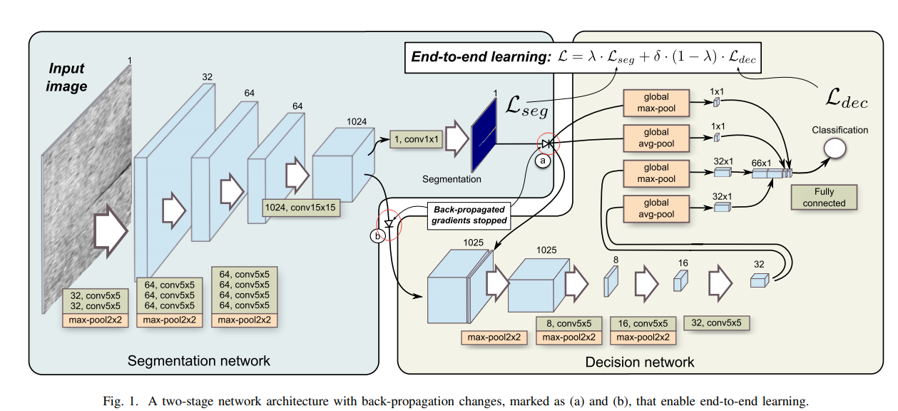
We propose to eliminate the gradient-flow from the classification network through the segmentation network, which is required to successfully learn the segmentation and the classification layers in a single endto-end manner. First, we remove the gradient-flow through the max/avg-pooling shortcuts used by the classification network as proposed in [9]. In Figure 1, this is marked with the (a). Those shortcuts utilize the segmentation network’s output map to speed-up the classification learning. Propagating gradients back through them would add error gradients to the segmentation’s output map, however, this can be harmful since we already have error for that output in the form of pixel-level annotation.
我们提议通过分割网络来消除分类网络的梯度流,这个需要在一个简单的端对端方式中,分割网络和分类网络都能很好的学习。首先我们使用9中提到的在分类网络中使用max/avg-pooling裁剪溢出了梯度流。这些裁剪使用分割网络的输出图来增加分类网络训练。梯度回传会给分割的输出图添加错误的梯度,这可能是有害的,因为我们已经有了以像素为对象的输出错误。
We also propose to limit the gradients for the segmentation that originate in the classification network. In Figure 1, this is marked with the (b). During the initial phases of the training, the segmentation net does not yet produce meaningful outputs, therefore gradients back-propagating from the classification network can negatively effect the segmentation part. We propose to completely stop those gradients, thus preventing the classification network from changing the segmentation network. This closely follows the behaviour of a two-stage learning from [9], where segmentation network is trained first, then the segmentation layers are frozen and only the classification network is trained in the end.
我们也提议在分割中限制起源于分类网络的梯度。在第一幅图中,在初始化参数的训练中,分割网络无法产生有意义的输出,因此来自于分类网络的梯度回传可能有害于分割部分。我们提议完全禁止这些梯度,因此预防分类网络改变分割网络。这和9中的2步训练方式有些接近,首先训练分割网络,然后分割网络被冻结,在最后的时候只训练分类网络
------------恢复内容开始------------
这篇文章相比于Segmentation-based deep- ˇ learning approach for surface-defect detection.这篇文章,首先他们都是一个作者写的,其次网络的架构也是非常接近的
为了保证小细节被保留下来,这里使用的是max-pool2x2,而不是使用stride=2的卷积,这里使用了3次的max-pool2x2, 用来构成分割的主体网络,从图中可以看出,Segmentation结果相比于原始图小了8倍,因此这里使用的分割标签low-level resolution,粗略的标签而不是精细的标签,因为作者认为相比于像素集的损失,判断是否有缺陷的分类结果更为重要。

这里讲一下文章中所提到的四个关键优化点
1. Dynamically balanced loss
To implement end-to-end learning, we combine both losses, the segmentation loss and the classification loss, into a single unified loss, allowing for a simultaneous learning. New combined loss is defined as:
为了使用端到端的学习,我们融合了两种Loss, 分割loss和分类的loss,融合为一种简单统一loss,允许进行共同学习。新的loss如下:

where Lseg and Lcls represent segmentation and classification losses, respectively, δ is an additional classification loss weight that prevents the classification loss from dominating the total loss, while λ is a mixing factor that balances the contribution of each network in the final loss. Note that λ, and δ do not replace the learning rate η in SGD, but complement it. They adequately control the learning process, as losses can be in different scales. The segmentation loss is averaged over all the pixels, and more importantly, only a handful of pixels are anomalous, resulting in a relatively small values compared to the classification loss, therefore we normally use smaller δ values to prevent the classification loss from dominating the total loss.
这里Lseg和Lcls表示分割和分类的loss,各自的,δ是一个额外的分类损失权重这可以防止分类的loss占据总的Loss,λ是一个混合因子可以平衡不同网络在最终loss中的贡献。注意,λ, and δ不能替换SGD中的学习率,但是可以补充它。他们充分的控制着学习流程,作为在不同尺寸上的损失。这个Segmentation loss 是相对于所有像素的平均,更加重要,但是只有少了的像素值是目标,相比于分类损失这个数值就很小,因此我们使用一个更小的δ 数值来预防分类损失占据整个损失。
损失函数结构:
weight_loss_seg * loss_seg + weight_loss_dec * loss_dec
Learning the classification network before the segmentation network features are stable represents an additional challenge for the simultaneous learning. We address this by proposing to start learning only the segmentation network at the beginning and gradually progress towards learning only the classification part at the end. We formulate this by computing segmentation and classification mixing factors as a simple linear function:
在分割网络特征稳定前训练分类网络对于同时训练是另外一个挑战。我们处理这情况通过在开始的时候训练分割网络并且逐步学习在最后的时候训练分类网络。我们制定这个通过计算分割和分类的混合因子作为一个简单的线性函数

其中λ等于1 - (epoch / total_epochs), δ等于self.cfg.DELTA_CLS_LOSS
    def get_loss_weights(self, epoch):
        total_epochs = float(self.cfg.EPOCHS)

        if self.cfg.DYN_BALANCED_LOSS:
            seg_loss_weight = 1 - (epoch / total_epochs)
            dec_loss_weight = self.cfg.DELTA_CLS_LOSS * (epoch / total_epochs)
        else:
            seg_loss_weight = 1
            dec_loss_weight = self.cfg.DELTA_CLS_LOSS

        self._log(f"Returning seg_loss_weight {seg_loss_weight} and dec_loss_weight {dec_loss_weight}", LVL_DEBUG)
        return seg_loss_weight, dec_loss_weight
where n represents the index of the current epoch and total epoch represents the total number of training epochs. Without the gradual mixing of both losses, the learning would in some cases result in exploding gradients, thus making the model more difficult to use. We term the process of gradually including classification network and excluding segmentation network as a dynamically balanced loss. Additionally, using lower δ values further reduces the issue of learning on the noisy segmentation features early on, whereas using greater values has sometimes lead to the problem of exploding gradients.
这里n表示当前的epoch的索引值,total epoch 表示整个训练的epoch次数,没有两种损失函数的逐步混合,这个训练将会在一些情况下导致梯度爆炸,因此导致这个网络更加难以使用。我们把这个逐步包括分类网络且不包含分割网络的过程称为动态平衡损失函数,另外,进一步使用较低的δ values减少在早期学习到带有噪声的分割特征,然而使用较大的值有时候会导致梯度爆炸的问题
2.Gradient-flow adjustments
We propose to eliminate the gradient-flow from the classification network through the segmentation network, which is required to successfully learn the segmentation and the classification layers in a single endto-end manner. First, we remove the gradient-flow through the max/avg-pooling shortcuts used by the classification network as proposed in [9]. In Figure 1, this is marked with the (a). Those shortcuts utilize the segmentation network’s output map to speed-up the classification learning. Propagating gradients back through them would add error gradients to the segmentation’s output map, however, this can be harmful since we already have error for that output in the form of pixel-level annotation.
我们提议通过分割网络来消除分类网络的梯度流,这个需要在一个简单的端对端方式中,分割网络和分类网络都能很好的学习。首先我们使用9中提到的在分类网络中使用max/avg-pooling裁剪溢出了梯度流。这些裁剪使用分割网络的输出图来增加分类网络训练。梯度回传会给分割的输出图添加错误的梯度,这可能是有害的,因为我们已经有了以像素为对象的输出错误。
We also propose to limit the gradients for the segmentation that originate in the classification network. In Figure 1, this is marked with the (b). During the initial phases of the training, the segmentation net does not yet produce meaningful outputs, therefore gradients back-propagating from the classification network can negatively effect the segmentation part. We propose to completely stop those gradients, thus preventing the classification network from changing the segmentation network. This closely follows the behaviour of a two-stage learning from [9], where segmentation network is trained first, then the segmentation layers are frozen and only the classification network is trained in the end.
我们也提议在分割中限制起源于分类网络的梯度。在第一幅图中,在初始化参数的训练中,分割网络无法产生有意义的输出,因此来自于分类网络的梯度回传可能有害于分割部分。我们提议完全禁止这些梯度,因此预防分类网络改变分割网络。这和9中的2步训练方式有些接近,首先训练分割网络,然后分割网络被冻结,在最后的时候只训练分类网络
这里禁止了两个红色框出来的梯度回传,即cat成1025以后的梯度和global max-pool以及global avg-pool, 使用的方式是通过给回传的梯度设置一个0的权重,即相乘以后的梯度为0。
self.volume_lr_multiplier_layer = GradientMultiplyLayer().apply
self.glob_max_lr_multiplier_layer = GradientMultiplyLayer().apply
self.glob_avg_lr_multiplier_layer = GradientMultiplyLayer().apply

cat = self.volume_lr_multiplier_layer(cat, self.volume_lr_multiplier_mask) # 给cat层添加一个梯度层
global_max_seg = self.glob_max_lr_multiplier_layer(global_max_seg, self.glob_max_lr_multiplier_mask) # 给global_max_seg设置梯度层
global_avg_seg = self.glob_avg_lr_multiplier_layer(global_avg_seg, self.glob_avg_lr_multiplier_mask) # 给global_avg_seg设置梯度层

class GradientMultiplyLayer(torch.autograd.Function):
    @staticmethod
    def forward(ctx, input, mask_bw):
        ctx.save_for_backward(mask_bw) #将mask_bw 进行保存
        return input

    @staticmethod
    def backward(ctx, grad_output):
        mask_bw, = ctx.saved_tensors # 取出tensors的结果
        return grad_output.mul(mask_bw), None # 将梯度与结果进行回传
3.Frequency-of-use sampling
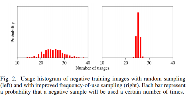
Current implementation of the two-stage architecture employed an alternating sampling scheme [9] that provided balance between the positive and the negative training samples by alternating between a positive and a negative sample in each training step. We propose to improve the alternating sampling scheme by replacing the naive random sampling with one based on the frequency of use of each negative sample. The existing alternating sampling scheme forces a selection of negative images (N˜ ⊂ N) for every epoch in the same amount of positive images (P). However, due too P << N, the selected subset N˜ will be relatively small. Since current approach [9] employs uniform random sampling of negative images for every epoch, this leads to a significant over-use of some samples and under-use of others, as can be observed on the left side in Figure 2.
两阶段结构的当前实现采用一个交替抽样的方案,这个方案通过在每一个训练步中选择一个正样本还是一个负样来提供正样本和负样本之间的平衡。我们提出了一种改进的交替抽样的方案,通过基于每一个负样本的使用频率来替换掉单纯的随机抽样。现有的交替抽样方案在等量的正样本中迫使选择一个负样本,然而,归结于P<<N, 可选择N的子集相比而言要少,因此每个epoch中,当前的方法采用统一随机抽取负样本,这将会导致一些样本的过度使用和其他样本的使用不足,这个可以在左上角的figure2观察到。
We propose to replace the random sampling of negative examples with a one based on the frequency-of-use. We sample each image with the probability inversely proportional to the frequency of use of that image. As seen in the right histogram in Figure 2, the frequency-of-use sampling significantly reduces the over-use and the under-use in all samples, and ensures even use of every negative image during the training process.
我们打算使用基于概率使用的方法来替换随机抽取负样本。我们采样每一张图片的概率与这张图片的使用频率成反比,这种概率的采样可以很好的降低过度使用和使用不足的情况,并且可以确保在训练过程中每一个负样本的使用。
当迭代的次数self.counter小于self.len的时候,负样本(没有缺陷的)的使用个数与正样本(有缺陷的)的使用个数相同, 在2x正样本的个数中抽取数据。即最前面的正样本的个数的负样本被抽取到
当迭代的次数self.counter大于self.len的时候, 即经过了一个epoch,重新对负样本的索引进行随机抽取,已经被抽取到的负样本的概率减少,没有被抽取到的负样本的概率增加
上述的好处,1. 每一个epoch过程中,正样本和负样本的个数是一样的
2.每一个负样本被抽取的概率是接近的。
个人理解,在样本量比较少的时候,这种方法是有效的,样本量比较大的时候,采用随机抽取也是有效的。
 if self.counter >= self.len: # 刚开始不进入
    self.counter = 0
    if self.frequency_sampling:
          sample_probability = 1 - (self.neg_retrieval_freq / np.max(self.neg_retrieval_freq)) # 将1变为0, 0变为1
          sample_probability = sample_probability - np.median(sample_probability) + 1 # 计算其中值
          sample_probability = sample_probability ** (np.log(len(sample_probability)) * 4)
          sample_probability = sample_probability / np.sum(sample_probability)

          # use replace=False for to get only unique values
          self.neg_imgs_permutation = np.random.choice(range(self.num_neg),
                                                       size=self.num_negatives_per_one_positive * self.num_pos,
                                                       p=sample_probability,
                                                       replace=False) # p是用来保证抽取的概率, 即已经抽取过的概率要小
            else:
                self.neg_imgs_permutation = np.random.permutation(self.num_neg)


if self.kind == 'TRAIN':
    if index >= self.num_pos: # 79
          ix = index % self.num_pos
          ix = self.neg_imgs_permutation[ix] # 选择72
          item = self.neg_samples[ix]
          self.neg_retrieval_freq[ix] = self.neg_retrieval_freq[ix] + 1 # 将其中挑选的负样本标记为1

    else:
          ix = index
          item = self.pos_samples[ix]
else:
    if index < self.num_neg:
          ix = index
          item = self.neg_samples[ix]
    else:
          ix = index - self.num_neg
          item = self.pos_samples[ix]
4. Loss weighting for positive pixels
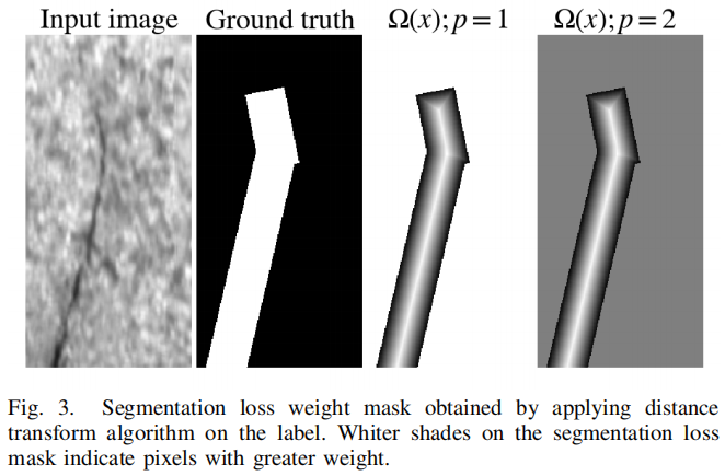
When only approximate, region-based labels are available, such as shown in Figure 3, we propose to consider the different pixels of the annotated defected regions differently. In particular, we give more importance to the center of the annotated regions and less importance to the outer parts. This alleviates the ambiguity arising at the edges of the defect, where we can not be certain whether the defect is present or not. We implement the importance in different sections of labels by weighting the segmentation loss accordingly. We weight the influence of each pixel at positive labels in accordance with its distance to the nearest negatively labelled pixel using the distance transform algorithm.
We formulate weighting of the positive pixels as:

当只有近似,基于区域的标签是有效的,就像Figure3图中显示的,我们建议对不同标注区域的像素点进行不同的考虑,特别的,我们对于目标区域给出更多关注和给外部区域更少的关注。这将会减少在缺陷边界的不确定性,当我们不能确定缺陷 是否是存在的。我们直接通过加权分割的损失来实现标签不同位置的重要性。我们使用距离变化方法,根据离最近负标签像素的距离,来对每一个正样本的像素进行加权。
where Lˆ(pix) is the original loss of the pixel, D(pix)/D(pixmax) is a distance to the nearest negative pixel normalized by the maximum distance value within the groundtruth region and Ω(x) is a scaling function that converts the relative distance value into the weight for the loss. In general, the scaling function Ω(x) can be defined differently depending on the defect and annotation type. However, we have found that a simple polynomial function provides enough flexibility for different defect types:
这里L^(pix)是一个原始的像素loss,D(pix) / D(pixmax)是由在真实样本区域内最大距离归一化到最近负样本像素的距离,Ω(x)是一个缩放函数,它将将相对的距离转换为损失权重,缩放函数Ω(x)可以根据缺陷和目标的类型被定义为不同。然而,我们发现简单的线性函数可以表达出足够的灵活性来应对不同的缺陷类型

where p controls the rate of decreasing the pixel importance as it gets further away from the center, while wpos is an additional scalar weight for all positive pixels. We have often found p = 1 and p = 2 as best performing, depending on the annotation type. Examples of a segmentation mask and two weight masks are depicted in Figure 3. Note, that the weights for the negatively labeled pixels remain 1.
这里p控制着像素的重要性随着其远离中心点而降低的速度,这里wpos是一个额外的权重对于所有的正像素。我们发现p=1和p=2拥有最好的表现,取决于注释的类型。一个分割的掩模和两个权重的掩模在Figure3被展示,注意,对于负样本像素的标签这个权重使用保持为1.
对分割的loss根据非零点到最近零点的距离计算,作为分割损失的加权,使得中心位置的权重大于边缘位置,可以提高边界的分界情况。
 def distance_transform(self, mask: np.ndarray, max_val: float, p: float) -> np.ndarray:
        h, w = mask.shape[:2] # label max_val = 1 p = 2
        dst_trf = np.zeros((h, w))

        num_labels, labels = cv2.connectedComponents((mask * 255.0).astype(np.uint8), connectivity=8) #相邻的缺陷聚集为一个类别
        for idx in range(1, num_labels): #
            mask_roi= np.zeros((h, w))
            k = labels == idx #找出标签等于类别的位置
            mask_roi[k] = 255 # 将其中等于类别的位置设置为255
            dst_trf_roi = distance_transform_edt(mask_roi) #计算非零点到最近零点的距离,此时边界的权重为1,靠近中心的位置大于1,且越靠近中心值越大
            if dst_trf_roi.max() > 0: # 如果存在这样的结果
                dst_trf_roi = (dst_trf_roi / dst_trf_roi.max())
                dst_trf_roi = (dst_trf_roi ** p) * max_val # max_val 表示Wpos
            dst_trf += dst_trf_roi # 将结果进行相加

        dst_trf[mask == 0] = 1 # 将负样本的标签权重设置为1
        return np.array(dst_trf, dtype=np.float32)
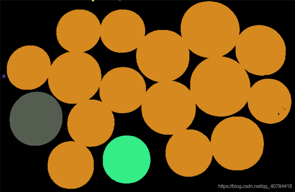
上述函数说明: cv2.connectedComponents((mask * 255.0).astype(np.uint8), connectivity=8),这里实现的效果如下 将相连的像素分割为一类
原始图 效果图

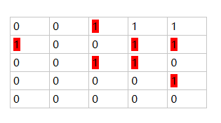
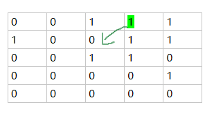
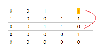
上述函数说明: distance_transform_edt计算非零像素到最近的零像素的距离
离最近背景点距离为1的用红色标出,如下图所示
离最近背景点距离为sqrt(2)
离最近背景点距离为2 的用橘色标出,如下图所示


 浙公网安备 33010602011771号