Python Matplotlib绘制柏拉图以及在ax.table上绘制矩形、直线、椭圆
个人示例
Bar
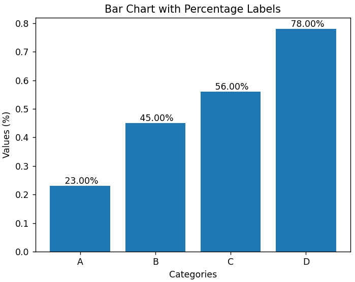
垂直柱状图
创建一个柱状图,并且在每个柱子的上方显示百分比:
代码实现:
import matplotlib.pyplot as plt
# 示例数据
categories = ['A', 'B', 'C', 'D']
values = [0.23, 0.45, 0.56, 0.78]  # 这些值将被转换为百分数
# 创建一个figure和axes
fig, ax = plt.subplots()
# 绘制柱状图
bars = ax.bar(categories, values)
# 为每个柱子添加标签,将值转换为百分数
ax.bar_label(bars, labels=[f' {val*100:.2f}%' for val in values])
# 设置标题和标签
ax.set_title('Bar Chart with Percentage Labels')
ax.set_xlabel('Categories')
ax.set_ylabel('Values (%)')
# 显示图表
plt.show()
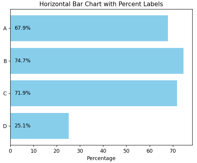
水平柱状图
创建一个水平柱状图,并且在柱子的底部显示百分比:
import matplotlib.pyplot as plt
import numpy as np

# 示例数据
categories = ['A', 'B', 'C', 'D']
values = np.random.rand(4)  # 生成0到100之间的随机小数
# 创建一个figure和axes
fig, ax = plt.subplots()
# 绘制水平柱状图
bars = ax.barh(categories, values, color='skyblue')
ax.bar_label(bars, labels=[f' {val*100:.2f}%' for val in values])
# 设置标题和标签
ax.set_title('Horizontal Bar Chart with Percent Labels')
ax.set_xlabel('Percentage')
# 显示图表
plt.show()
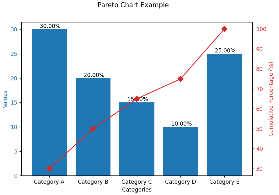
柏拉图
红色的为累加百分比,柱状图为每个类型的值。
代码:
import matplotlib.pyplot as plt
import numpy as np

# 示例数据:分类和对应的值
categories = ['Category A', 'Category B', 'Category C', 'Category D', 'Category E']
values = [30, 20, 15, 10, 25]
# 计算累积和
cumulative_values = np.cumsum(values)
# 计算累积百分比
cumulative_percentages = cumulative_values / cumulative_values[-1] * 100
percentages = []
# 遍历列表,计算并打印每个元素的百分比
for number in values:
    percentages.append((number / sum(values)))
# 创建图形和坐标轴
fig, ax1 = plt.subplots()
# 绘制柱状图
color = 'tab:blue'
ax1.set_xlabel('Categories')
ax1.set_ylabel('Values', color=color)
bars = ax1.bar(categories, values, color=color)
ax1.bar_label(bars, labels=[f' {val*100:.2f}%' for val in percentages])
ax1.tick_params(axis='y', labelcolor=color)
# 绘制累积百分比的折线图
ax2 = ax1.twinx()  # 创建共享x轴的第二个y轴
color = 'tab:red'
ax2.set_ylabel('Cumulative Percentage (%)', color=color)
ax2.plot(categories, cumulative_percentages, color=color, marker='D', ms=7, linestyle='-')
ax2.tick_params(axis='y', labelcolor=color)
# 设置图表标题
fig.suptitle('Pareto Chart Example')
# 显示图形
plt.show()
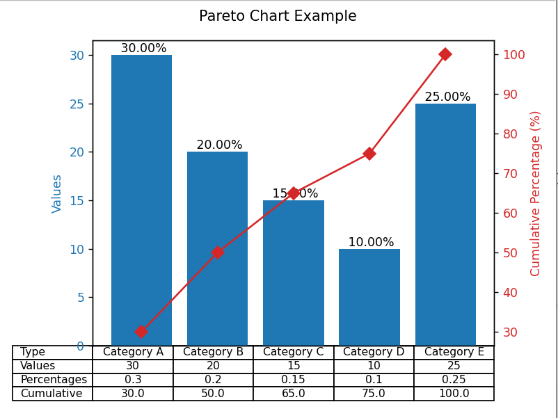
改进:在柏拉图下方显示一个table
import matplotlib.pyplot as plt
import numpy as np

# 示例数据:分类和对应的值
categories = ['Category A', 'Category B', 'Category C', 'Category D', 'Category E']
values = [30, 20, 15, 10, 25]
cumulative_values = np.cumsum(values)   # 计算累积和
cumulative_percentages = cumulative_values / cumulative_values[-1] * 100    # 计算累积百分比
percentages = []
for number in values:   # 遍历列表,计算并打印每个元素的百分比
    percentages.append((number / sum(values)))
# 创建图形和坐标轴
fig, ax1 = plt.subplots()
# 绘制柱状图
color = 'tab:blue'
ax1.set_ylabel('Values', color=color)
bars = ax1.bar(categories, values, color=color)
ax1.bar_label(bars, labels=[f' {val*100:.2f}%' for val in percentages])
ax1.tick_params(axis='y', labelcolor=color)
# 绘制累积百分比的折线图
ax2 = ax1.twinx()  # 创建共享x轴的第二个y轴
color = 'tab:red'
ax2.set_ylabel('Cumulative Percentage (%)', color=color)
ax2.plot(categories, cumulative_percentages, color=color, marker='D', ms=7, linestyle='-')
ax2.tick_params(axis='y', labelcolor=color)
# 添加table
cell_text = [categories, values, percentages, cumulative_percentages]
columns = ["Type", "Values", "Percentages", "Cumulative"]
ax1.table(cellText=cell_text, rowLabels=columns, loc='bottom', cellLoc='center')
plt.xticks([])
plt.subplots_adjust(left=0.2, bottom=0.1)
fig.tight_layout()
# 设置图表标题
fig.suptitle('Pareto Chart Example')
plt.tight_layout()
# 显示图形
plt.show()
轴坐标
在 Matplotlib 中,轴坐标(也称为归一化坐标)是一种特殊的坐标系统,它用于相对于当前轴(Axes)的位置和大小来定位图形元素。轴坐标的范围是从 0 到 1,其中 (0, 0) 表示轴的左下角,(1, 1) 表示轴的右上角。这种坐标系统不依赖于数据的实际值或图形的物理尺寸,而是基于轴的可视化区域。
使用轴坐标可以方便地放置图形元素,如标题、图例、注释或自定义的图形(如矩形、圆形等),而无需担心数据范围或图形窗口大小的变化。这是因为轴坐标是相对于轴的可视化区域进行解释的,而不是相对于数据或图形窗口的像素尺寸。
在 Matplotlib 中,你可以通过传递 transform=ax.transAxes 参数给图形元素(如 Rectangle、Text 等)来指定使用轴坐标。ax 是你的 Axes 对象,而 transAxes 是该轴对象的一个属性,表示轴坐标变换。
在table上绘制图形和线条
ax.table创建的时候,使用的是轴坐标系统,但是ax.table的get_window_extent()方法返回的是像素坐标,而不是轴坐标:
bbox = the_table.get_window_extent()
x0, y0 = bbox.x0, bbox.y0  				# 获取左下角的坐标
width, height = bbox.width, bbox.height # 获取宽度和高度
下面讲解在ax.table上绘制各种图形时的坐标系统:
-
Rectangle:绘制矩形,使用的是轴坐标系统
# : +------------------+ # : | | # : height | # : | | # : (xy)---- width -----+ class matplotlib.patches.Rectangle(xy, width, height, *, angle=0.0, rotation_point='xy', **kwargs) -
axhline:绘制水平直线,使用的是轴坐标系统
''' y: 水平线的数据坐标中的y位置, 使用的是像素坐标系 xmin: 应介于0和1之间,0表示绘图的最左侧,1表示绘图的最右侧, 使用的是轴坐标系。 xmax: 应介于0和1之间,0表示绘图的最左侧,1表示绘图的最右侧, 使用的是轴坐标系。 ''' Axes.axhline(y=0, xmin=0, xmax=1, **kwargs) -
axvline:绘制垂直线,使用的是轴坐标系统
''' x: 垂直线的数据坐标中的x位置, 使用的是像素坐标系 ymin: 应介于0和1之间,0是绘图的底部,1是绘图的顶部, 使用的是轴坐标系。 ymax: 应介于0和1之间,0是绘图的底部,1是绘图的顶部, 使用的是轴坐标系。 ''' Axes.axvline(x=0, ymin=0, ymax=1, **kwargs) -
Ellipse:绘制椭圆,使用的是像素坐标系统
# xy: 椭圆中心的 xy 坐标
# width: 长轴的总长度
# height: 短轴的总长度
class matplotlib.patches.Ellipse(xy, width, height, *, angle=0, **kwargs)
以下是一个举例,创建一个table,然后在上面绘制水平直线、垂直直线、矩形、椭圆形:
实现代码:
import matplotlib.pyplot as plt
from matplotlib.patches import Rectangle
from matplotlib.patches import Ellipse
from matplotlib.backends.backend_agg import FigureCanvasAgg as FigureCanvas
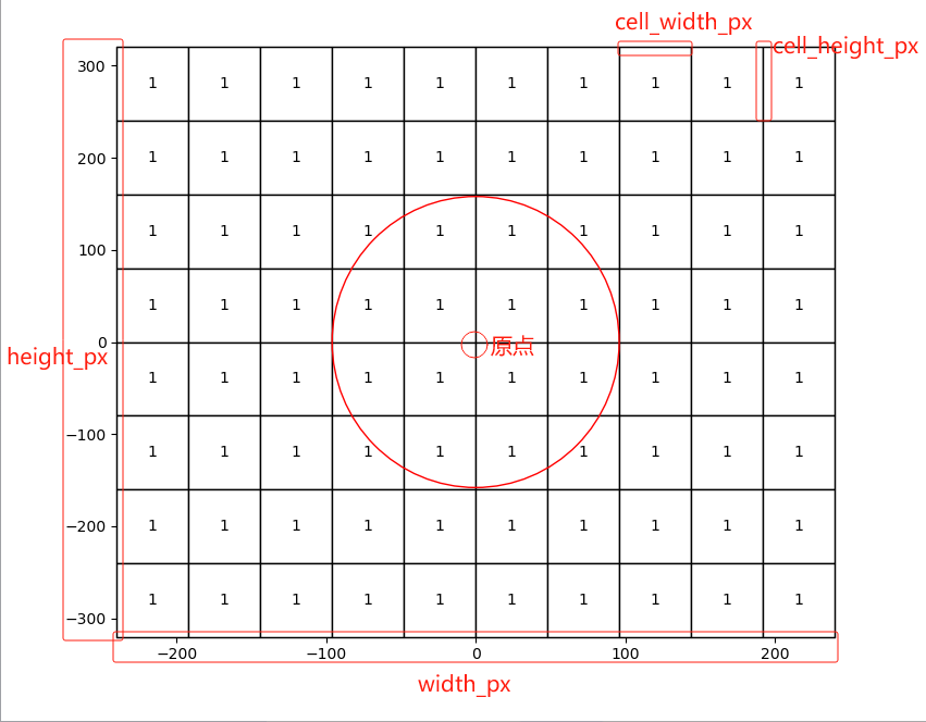
cell_width_px = 0
cell_height_px = 0
width_px = 0
height_px = 0
# 对于像素坐标系统,需要计算每个Cell的宽度和高度
def calculate_cell_size(fig, num_rows, num_cols):
global width_px
global height_px
global cell_width_px
global cell_height_px
# 绘制椭圆图形(这一步是必需的,以便FigureCanvas可以捕获渲染后的图形)
fig.canvas.draw()
# 获取FigureCanvas对象(这里我们假设使用的是Agg后端,但你可以根据你的后端进行调整)
canvas = FigureCanvas(fig)
# 获取图形的宽度和高度(以像素为单位)
width_px, height_px = canvas.get_width_height()
# 估算每个单元格的像素宽度和高度, 减去边距、标签等
cell_width_px = width_px / num_cols - 16 # 16只是人为估计出来的误差
cell_height_px = height_px / num_rows + 19 # 19只是人为估计出来的误差
print(f"Estimated width in pixels: {width_px}")
print(f"Estimated height in pixels: {height_px}")
print(f"Estimated cell width in pixels: {cell_width_px}")
print(f"Estimated cell height in pixels: {cell_height_px}")
# x0, y0, x1, y1代表的是cell的位置
# : +------------------+
# : | |
# : height |
# : | |
# : (xy)---- width -----+
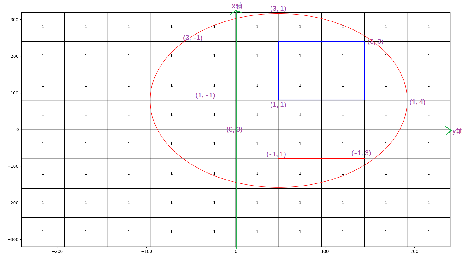
def draw_rectangle(ax, rows, columns, xy, width, heights):
# 由于创建表时已经设置了轴坐标范围为(0, 0)->(1, 1), 因此计算单个cell的宽和高就很方便
cell_width = 1 / columns
cell_height = 1 / rows
# 由于表格中央被我们当作坐标原点, 但是极坐标的坐标原点默认为左下角, 因此需要添加一个偏移
start_x = (xy[1] + columns / 2 )* cell_width
start_y = (xy[0] + rows / 2) * cell_height
rect_width = width * cell_width
rect_height = heights * cell_height
print (start_x, start_y, rect_width, rect_height)
rect = Rectangle((start_x, start_y), rect_width, rect_height, linewidth=1.5,
edgecolor='blue', facecolor='none', transform=ax.transAxes)
ax.add_patch(rect)
# 绘制椭圆形
# xy: 椭圆原点(x, y)
# width: 水平轴直径
# height: 垂直轴执行
def draw_ellipse(ax, xy, width, height):
ellipse_width = cell_width_px * width # 水平轴
ellipse_height = cell_height_px * height # 垂直轴
x1 = xy[0] * cell_width_px
y1 = xy[1] * cell_height_px
ellipse = Ellipse((x1, y1), ellipse_width, ellipse_height, edgecolor='red', facecolor='none')
ax.add_patch(ellipse)
# 在轴上添加一个水平线: matplotlib.pyplot.axhline(y=0, xmin=0, xmax=1, **kwargs)
# '''
# : +--------------------+
# : | |
# (x0, y0) +----------- y1 -----+
# : | |
# : +--------------------+
# '''
def draw_axhline(ax, columns, x0, y0, y1):
cell_width = 1 / columns # 创建表时已经设置了轴坐标范围为(0, 0)->(1, 1)
y = x0 * cell_height_px # 使用的是数据(像素)坐标系
x_min = (y0 + columns / 2) * cell_width # 使用的是轴坐标系
x_max = (y1 + columns / 2) * cell_width # 使用的是轴坐标系
print (y, x_min, x_max)
ax.axhline(y, x_min, x_max, linewidth=1.5, color='red')
# 在轴上添加一条垂直线: Axes.axvline(x=0, ymin=0, ymax=1, **kwargs)
# '''
# : y1-------------------+
# : | |
# : |--------------------+
# : | |
# :(x0, y0) +--------------------+
# '''
def draw_axvline(ax, rows, y0, x0, x1):
cell_height = 1 / rows # 创建表时已经设置了轴坐标范围为(0, 0)->(1, 1)
x = y0 * cell_width_px # 使用的是数据(像素)坐标系
y_min = (x0 + rows / 2) * cell_height # 使用的是轴坐标系
y_max = (x1 + rows / 2) * cell_height # 使用的是轴坐标系
print (x, y_min, y_max)
ax.axvline(x, y_min, y_max, linewidth=2, color='cyan')
if __name__ == '__main__':
rows = 8
columns = 10
cell_text = [[1 for x in range(columns)] for y in range(rows)]
fig, ax = plt.subplots()
the_table = ax.table(
cellText=cell_text,
loc='center', cellLoc='center',
bbox=[0, 0, 1, 1], # 为了方便, 将轴坐标范围设置为[0, 0]->[1, 1]
edges = 'closed',
)
calculate_cell_size(fig, rows, columns)
# 将坐标原点设置到table的中央
ax.set_xlim(-height_px/2, height_px/2) # 设置坐标轴原点
ax.set_ylim(-width_px/2, width_px/2) # 设置坐标轴原点
# 绘图
draw_rectangle(ax, rows, columns, (1, 1), 2, 2)
draw_ellipse(ax, (1, 1), 6, 6)
draw_axhline(ax, columns, -1, 1, 3)
draw_axvline(ax, rows, -1, 1, 3)
plt.show()
实现效果:

 浙公网安备 33010602011771号