使用R包SpATS消除植物育种中田间试验的空间异质性
简介
R包SpATS (Spatial Analysis of field Trials with Splines) 通过使用P-splines方法,校正植物育种田间试验中的空间异质性,如不同田间地块的管理措施(施肥打药等)或其他各种不稳定的空间趋势带来的影响。
以使用二维(2-D)平滑表面模拟随机空间变化,对样本、田块、重复和/或其他空间变化因素建立混合模型,该模型的特点:
- 对田间(field)的空间趋势有详尽的估计;
- 估计稳定快速;
- 易处理大量缺失的小区(plots);
- 易扩展非正态响应。
原理和公式推导比较费劲,有能力直接看文章吧:
Rodriguez-Alvarez, M.X, Boer, M.P., van Eeuwijk, F.A., and Eilers, P.H.C. (2018). Correcting for spatial heterogeneity in plant breeding experiments with P-splines. Spatial Statistics, 23, 52 - 71. https://doi.org/10.1016/j.spasta.2017.10.003.
Demo测试
1. 数据说明
library(SpATS)
data(wheatdata)
summary(wheatdata)
?wheatdata
完全区组设计试验。107个品种geno,3个重复(每个播2次),每个重复由5列22行组成,因此共330个观测值yield(15列col x 22行row),rowcode和colcode分别是行列不同走位方式。
  yield geno rep row col rowcode colcode
1   483    4   1   1   1       2       1
2   526   10   1   2   1       2       1
3   557   17   1   3   1       1       1
4   564   16   1   4   1       2       1
5   498   21   1   5   1       2       1
6   510   32   1   6   1       1       1
数据更详细信息见:
Gilmour, A.R., Cullis, B.R., and Verbyla, A.P. (1997). Accounting for Natural and Extraneous Variation in the Analysis of Field Experiments. Journal of Agricultural, Biological, and Environmental Statistics, 2, 269 - 293.
2. 建模测试
固定效应或随机效应,可根据试验自己设定。
# Create factor variable for row and columns
wheatdata$R <- as.factor(wheatdata$row)
wheatdata$C <- as.factor(wheatdata$col)

m0 <- SpATS(response = "yield", #拟合响应变量,即性状名
            spatial = ~ SAP(col, row, nseg = c(10,20), degree = 3, pord = 2), #P-Spline模型公式
            genotype = "geno", #品种/样本名(我也不知道老外为何总喜欢用genotype)
            fixed = ~ colcode + rowcode, #固定效应
            random = ~ R + C, #随机效应
            data = wheatdata, #数据
            control =  list(tolerance = 1e-03)) #控制 SpATS 模型估计的一些默认参数(这里tolerance收敛标准容差)
3. 结果
结果汇总:
# Brief summary
> m0

Spatial analysis of trials with splines

Response:                   yield
Genotypes (as fixed):       geno
Spatial:                    ~SAP(col, row, nseg = c(10, 20), degree = 3, pord = 2)
Fixed:                      ~colcode + rowcode
Random:                     ~R + C


Number of observations:        330
Number of missing data:        0
Effective dimension:           149.05
Deviance:                      2065.824


# More information: dimensions
> summary(m0)

Spatial analysis of trials with splines

Response:                   yield
Genotypes (as fixed):       geno
Spatial:                    ~SAP(col, row, nseg = c(10, 20), degree = 3, pord = 2)
Fixed:                      ~colcode + rowcode
Random:                     ~R + C


Number of observations:        330
Number of missing data:        0
Effective dimension:           149.05
Deviance:                      2065.824

Dimensions:
                      Effective     Model     Nominal     Ratio     Type
geno                      106.0       106         106      1.00        F
Intercept                   1.0         1           1      1.00        F
colcode                     3.0         3           3      1.00        F
rowcode                     1.0         1           1      1.00        F
R                           8.7        22          19      0.46        R
C                           6.8        15          10      0.68        R
col                         1.0         1           1      1.00        S
row                         1.0         1           1      1.00        S
rowcol                      1.0         1           1      1.00        S
f(col,row)|col             10.2        NA          NA        NA        S
f(col,row)|row              9.4        NA          NA        NA        S
f(col,row) Global          19.6       295         295      0.07        S

Total                     149.0       446         438      0.34
Residual                  181.0
Nobs                        330

Type codes: F 'Fixed'    R 'Random'    S 'Smooth/Semiparametric'

## More information: variances
#> summary(m0, which = "variances")
## More information: all
#> summary(m0, which = "all")
看看校正后的表型与原表型相关性:
> cor(wheatdata$yield,m0$fitted)
[1] 0.9773118
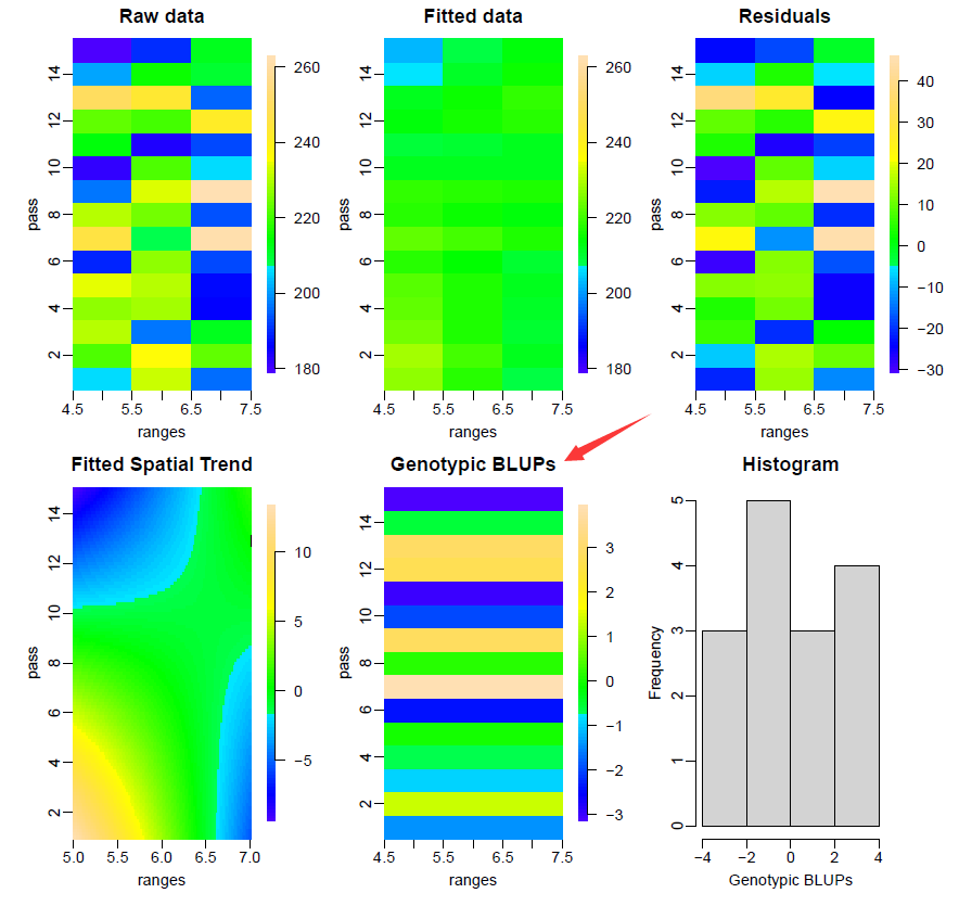
4. 可视化
# Plot results
plot(m0)
# plot(m0, all.in.one = FALSE)

这里品种/样本(genotype)作为固定效应,所以计算的是BLUE。
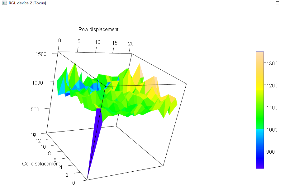
也可查看变异函数三维图(自由拖拽):
# Variogram
var.m0 <- variogram(m0)
plot(var.m0)
随机效应测试
完全随机的试验设计,可以把品种、行、列等都设为随机效应。
示例数据如下:
> head(data)
  loc_id ranges pass rep_num ped_id     Trait R  P
1   5052      5   15       1 44601 179.3017 5 15
2   5052      5    1       1 44604 206.0712 5  1
3   5052      5    2       1 44606 221.5142 5  2
4   5052      5    3       1 44607 230.8191 5  3
5   5052      5    4       1 44608 227.2715 5  4
6   5052      5    5       1 44609 235.0297 5  5
> str(data)
'data.frame':	180 obs. of  8 variables:
 $ loc_id : Factor w/ 4 levels "5052","5053",..: 1 1 1 1 1 1 1 1 1 1 ...
 $ ranges : int  5 5 5 5 5 5 5 5 5 5 ...
 $ pass   : int  15 1 2 3 4 5 6 7 8 9 ...
 $ rep_num: Factor w/ 3 levels "1","2","3": 1 1 1 1 1 1 1 1 1 1 ...
 $ Trait : Factor w/ 15 levels "44600","44601",..: 2 4 5 6 7 8 1 3 12 13 ...
 $ T002   : num  179 206 222 231 227 ...
 $ R      : Factor w/ 3 levels "5","6","7": 1 1 1 1 1 1 1 1 1 1 ...
 $ P      : Factor w/ 15 levels "1","2","3","4",..: 15 1 2 3 4 5 6 7 8 9 ...
利用SpATS建模:
M.fit<-SpATS(response = "Trait",
             spatial = ~ SAP(ranges, pass, nseg = c(10,20), degree = 3, pord = 2, nest.div=2),
             genotype = "ped_id",
             genotype.as.random = TRUE,
             random = ~ R + P,
             data = data,
             control =  list(tolerance = 1e-03))
这时的结果为BLUP:
Ref:
https://www.rdocumentation.org/packages/SpATS/versions/1.0-16/topics/SpATS
本文来自博客园,作者:生物信息与育种,转载请注明原文链接:https://www.cnblogs.com/miyuanbiotech/p/16296669.html。若要及时了解动态信息,请关注同名微信公众号:生物信息与育种。