[CV] 边缘提取和角点判断
两种方法:
- 一种直接沿着x轴和y轴方向求偏导
\[G_{x}=\frac{\partial f}{\partial x}, \quad G_{y}=\frac{\partial f}{\partial y}
\]
对应的边缘幅值:
\[A=\sqrt{G_{x}^{2}+G_{y}^{2}}
\]
边缘方向:
\[\phi=\arg \tan \left(\frac{G_{y}}{G_{x}}\right)-\frac{\pi}{2}
\]
- 抽取多个角度,选取偏导最大的方向(即等高线越紧密的地方越可能是边缘,计算公式和方法1类似)
算子
- 一阶差分算子Roberts算子
\[\frac{\partial f}{\partial x}=f(x, y)-f(x-1, y), \quad \frac{\partial f}{\partial y}=f(x, y)-f(x, y-1)
\]
因此卷积核通常取(45°和-45°):
\[h_{x}=\left[\begin{array}{cc}
-1 & 0 \\
0 & 1
\end{array}\right] \quad h_{y}=\left[\begin{array}{cc}
0 & -1 \\
1 & 0
\end{array}\right]
\]
-
一阶差分算子Prewitt算子
\[\begin{array}{ll} h_{x}=\left[\begin{array}{ccc} -1 & -1 & -1 \\ 0 & 0 & 0 \\ 1 & 1 & 1 \end{array}\right] & h_{y}=\left[\begin{array}{ccc} -1 & 0 & 1 \\ -1 & 0 & 1 \\ -1 & 0 & 1 \end{array}\right] \\ h_{45}=\left[\begin{array}{ccc} -1 & -1 & 0 \\ -1 & 0 & 1 \\ 0 & 1 & 1 \end{array}\right] & h_{135}=\left[\begin{array}{ccc} 0 & -1 & -1 \\ 1 & 0 & -1 \\ 1 & 1 & 0 \end{array}\right] \end{array} \] -
一阶差分Sobel算子(在正方向上的权值更大)
\[\begin{array}{ll} h_{x}=\left[\begin{array}{ccc} -1 & -2 & -1 \\ 0 & 0 & 0 \\ 1 & 2 & 1 \end{array}\right] & h_{y}=\left[\begin{array}{ccc} -1 & 0 & 1 \\ -2 & 0 & 2 \\ -1 & 0 & 1 \end{array}\right] \\ h_{45}=\left[\begin{array}{ccc} -2 & -1 & 0 \\ -1 & 0 & 1 \\ 0 & 1 & 2 \end{array}\right] & h_{135}=\left[\begin{array}{ccc} 0 & 1 & 2 \\ -1 & 0 & 1 \\ -2 & -1 & 0 \end{array}\right] \end{array} \] -
二阶拉普拉斯算子
\[\begin{array}{l}
\frac{\partial^{2} f}{\partial x^{2}}=f(x+1, y)+f(x-1, y)-2 f(x, y) \\
\frac{\partial^{2} f}{\partial y^{2}}=f(x, y+1)+f(x, y-1)-2 f(x, y)
\end{array}
\]
\[h=\left[\begin{array}{ccc}
0 & 1 & 0 \\
1 & -4 & 1 \\
0 & 1 & 0
\end{array}\right] \quad h=\left[\begin{array}{ccc}
1 & 1 & 1 \\
1 & -8 & 1 \\
1 & 1 & 1
\end{array}\right]
\]
提取边缘的算法描述:
- 使用一阶差分(两个相互垂直的方向)的算子进行卷积形成两幅差分图像
- 求两幅差分图像的对应点平方和开根号得幅值并使用设定的阈值[min,max]过滤得到边缘点
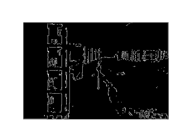
Canny 边缘提取
-
对图像做高斯卷积(平滑滤波)
# 边缘轮廓提取,Canny算法 # 进行高斯卷积计算 (rows,cols) = gray.shape # 定义高斯核 kernel = np.asarray([0.05,0.25,0.4,0.25,0.05]) gray = gray.astype(np.float64) # 先从x轴开始 x_axis = np.copy(gray) for row in range(rows): for col in range(2,cols-2): x_axis[row][col] = np.sum(np.multiply(gray[row,col-2:col+3].flatten(),kernel)) # 对y轴进行卷积 y_axis = np.copy(x_axis) for row in range(2,rows-2): for col in range(cols): y_axis[row][col] = np.sum(np.multiply(x_axis[row-2:row+3,col].flatten(),kernel)) gray = y_axis -
估计每个像素的边缘法向
# 利用Sobel算子计算x轴 x_kernel = np.asarray([[-1,0,1],[-2,0,2],[-1,0,1]]) x_axis = np.copy(gray) for row in range(1,rows-1): for col in range(1,cols-1): x_axis[row][col] = np.sum(np.multiply(gray[row-1:row+2,col-1:col+2],x_kernel)) # 计算y轴 y_kernel = np.asarray([[-1,-2,-1],[0,0,0],[1,2,1]]) y_axis = np.copy(gray) for row in range(1,rows-1): for col in range(1,cols-1): y_axis[row][col] = np.sum(np.multiply(gray[row-1:row+2,col-1:col+2],y_kernel)) s = np.sqrt(np.square(x_axis)+np.square(y_axis)) # 获取边缘法向估计 phi = np.arctan2(y_axis,x_axis) # 范围(-pi,pi) # 对边缘法向进行量化为八个方向 for row in range(rows): for col in range(cols): phi[row][col] = int((phi[row][col]+np.pi*2-np.pi/8)/(np.pi/8))%8 # 方向变换 -pi,pi 转为正常的0~2pi 然后再减去pi/8即(22.5°) phi = phi.astype(np.uint) -
用非最大抑制方法(Non-maximum Suppression)找到候选边缘点的位置,细化边缘
dirs = [(0,1),(1,1),(1,0),(1,-1),(0,-1),(-1,-1),(-1,0),(-1,1)] def inrange(row,col,rows,cols): if row<0 or col<0 or row>=rows or col>=cols: return False return True can = np.ones(phi.shape) # 定义幅值参数 t0 = 140 t1 = 150 assert t0<t1 q = queue.Queue() # 声明BFS队列 vis = np.ones(gray.shape) # 非最大抑制法 for row in range(rows): for col in range(cols): d = dirs[(phi[row][col]+2)%8] x,y = d[0]+row,d[1]+col value = s[row][col] # 取方向上的两个像素 if value<t1: can[row][col]=0 if value>t0: q.put((row,col)) # 如果大于t0则加入队列 vis[row][col]=0 else: if inrange(x,y,rows,cols) and s[x][y]>value: can[row][col] = 0 else: d = dirs[(phi[row][col]+6)%8] x,y = d[0]+row,d[1]+col if inrange(x,y,rows,cols) and s[x][y]>value: can[row][col] = 0 final = np.copy(can) -
计算候选边缘点的边缘幅度
-
做滞后阈值处理,消除虚假响应、形成连续边缘轮廓
# 滞后阈值处理
while not q.empty():
    (x,y) = q.get()
    for d in dirs:
        nxtx,nxty = x+d[0],y+d[1]
        # 若邻域有边缘,则该点也是边缘
        if inrange(nxtx,nxty,rows,cols) and final[nxtx][nxty]==1:
            final[x][y]=1
            break
    if final[x][y]==1:
        for d in dirs:
            nxtx,nxty = x+d[0],y+d[1]
            if inrange(nxtx,nxty,rows,cols) and final[nxtx][nxty]==0:
                value = s[nxtx][nxty]
                if value>t0 and value<t1 and vis[nxtx][nxty]==1:
                    vis[nxtx][nxty]=0
                    q.put((nxtx,nxty))
实验结果

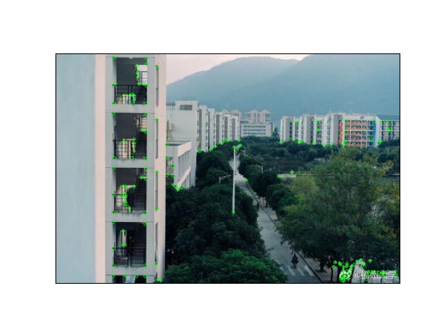
兴趣点提取
角点(corner)
-
Harris角点提取(博客园的步骤)
-
计算图像\(I(x,y)\)在\(X\)和\(Y\)两个方向的梯度\(I_x\)和\(I_y\)
\[I_{x}=\frac{\partial I}{\partial x}=I \otimes(-101), I_{y}=\frac{\partial I}{\partial x}=I \otimes(-101)^{T} \] -
计算图像两个方向的梯度乘积
\[I_{x}^{2}=I_{x} \cdot I_{y}, \quad I_{y}^{2}=I_{y} \cdot I_{y}, \quad I_{x y}=I_{x} \cdot I_{y} \] -
使用高斯函数对其进行高斯加权(即平滑滤波),生成矩阵A、B和C
\[A=g\left(I_{x}^{2}\right)=I_{x}^{2} \otimes w, C=g\left(I_{y}^{2}\right)=I_{y}^{2} \otimes w, B=g\left(I_{x, y}\right)=I_{x y} \otimes w \] -
计算每个像素的Harris响应值,并通过阈值过滤
-
在邻域内进行非最大抑制,局部最大值点即为图像中的角点
-
-
Harris角点提取(MOOC的步骤)
-
对图像进行高斯过滤
# Harris 角点提取 # 进行高斯卷积计算 (rows,cols) = gray.shape # 定义高斯核 kernel = np.asarray([0.05,0.25,0.4,0.25,0.05]) gray = gray.astype(np.float64) # 先从x轴开始 x_axis = np.copy(gray) for row in range(rows): for col in range(2,cols-2): x_axis[row][col] = np.sum(np.multiply(gray[row,col-2:col+3].flatten(),kernel)) # 对y轴进行卷积 y_axis = np.copy(x_axis) for row in range(2,rows-2): for col in range(cols): y_axis[row][col] = np.sum(np.multiply(x_axis[row-2:row+3,col].flatten(),kernel)) gray = y_axis -
对每个像素,估计其沿着x轴和y轴的一阶差分
# 利用Sobel算子计算x轴 x_kernel = np.asarray([[-1,0,1],[-2,0,2],[-1,0,1]]) x_axis = np.copy(gray) for row in range(1,rows-1): for col in range(1,cols-1): x_axis[row][col] = np.sum(np.multiply(gray[row-1:row+2,col-1:col+2],x_kernel)) # 计算y轴 y_kernel = np.asarray([[-1,-2,-1],[0,0,0],[1,2,1]]) y_axis = np.copy(gray) for row in range(1,rows-1): for col in range(1,cols-1): y_axis[row][col] = np.sum(np.multiply(gray[row-1:row+2,col-1:col+2],y_kernel)) -
对于每个像素和给定的邻域窗口,计算矩阵\(A(x,y)\),并计算响应矩阵函数\(R[A(x,y)]\),这里k一般选择为0.04~0.15
\[A(x, y)=\sum_{x_{i}, y_{i} \in W}\left[\begin{array}{ll} \left(\frac{\partial f}{\partial x}\right)^{2} & \frac{\partial f}{\partial x} \frac{\partial f}{\partial y} \\ \frac{\partial f}{\partial x} \frac{\partial f}{\partial y} & \left(\frac{\partial f}{\partial y}\right)^{2} \end{array}\right] \]\[R[A(x, y)]=\operatorname{det}[A(x, y)]-k \times \operatorname{trace}^{2}[A(x, y)] \]R = np.zeros(gray.shape) dirs = [(0,1),(1,1),(1,0),(1,-1),(0,-1),(-1,-1),(-1,0),(-1,1)] def inrange(row,col,rows,cols): if row<0 or col<0 or row>=rows or col>=cols: return False return True # k = 0.06 for row in range(rows): for col in range(cols): A = np.asarray([ [np.square(x_axis[row][col]),x_axis[row][col]*y_axis[row][col]], [x_axis[row][col]*y_axis[row][col],np.square(y_axis[row][col])] ]) for d in dirs: x,y = d[0]+row,d[1]+col if inrange(x,y,rows,cols): A=A+np.asarray([ [np.square(x_axis[x][y]),x_axis[x][y]*y_axis[x][y]], [x_axis[x][y]*y_axis[x][y],np.square(y_axis[x][y])] ]) det = np.linalg.det(A) trace = A.trace() R[row][col] = det/traceP.S. 这里使用是优化的比值公式,避免跨域太大的数值范围
-
设置一个\(R(A)\)的阈值,以此来选择最佳候选角点,用非最大化抑制来确定最终角点
final = np.ones(gray.shape)
maximum = R.max()
assert maximum>0
level = 0.2
for row in range(rows):
    for col in range(cols):
        if R[row][col]<level*maximum:
        # if R[row][col]>=maximum:
            final[row][col]=0
        else:
            for d in dirs:
                x,y = d[0]+row,d[1]+col
                if inrange(x,y,rows,cols) and R[x][y]>R[row][col]:
                    final[row][col]=0
                    break
final即为最后的角点位置
实验结果:
-
References:
