Use Pandas Groupby to Group and Summarise DataFrames
Pandas – Python Data Analysis Library
I’ve recently started using Python’s excellent Pandas library as a data analysis tool, and, while finding the transition from R’s excellent data.table library frustrating at times, I’m finding my way around and finding most things work quite well.
One aspect that I’ve recently been exploring is the task of grouping large data frames by different variables, and applying summary functions on each group. This is accomplished in Pandas using the “groupby()” and “agg()” functions of Panda’s DataFrame objects.
Update: Pandas version 0.20.1 in May 2017 changed the aggregation and grouping APIs. This post has been updated to reflect the new changes.
A Sample DataFrame

In order to demonstrate the effectiveness and simplicity of the grouping commands, we will need some data. For an example dataset, I have extracted my own mobile phone usage records. I analysed this type of data using Pandas during my work on KillBiller. If you’d like to follow along – the full csv file is available here.
The dataset contains 830 entries from my mobile phone log spanning a total time of 5 months. The CSV file can be loaded into a pandas DataFrame using the pandas.DataFrame.from_csv() function, and looks like this:
| date | duration | item | month | network | network_type | |
|---|---|---|---|---|---|---|
| 0 | 15/10/14 06:58 | 34.429 | data | 2014-11 | data | data |
| 1 | 15/10/14 06:58 | 13.000 | call | 2014-11 | Vodafone | mobile |
| 2 | 15/10/14 14:46 | 23.000 | call | 2014-11 | Meteor | mobile |
| 3 | 15/10/14 14:48 | 4.000 | call | 2014-11 | Tesco | mobile |
| 4 | 15/10/14 17:27 | 4.000 | call | 2014-11 | Tesco | mobile |
| 5 | 15/10/14 18:55 | 4.000 | call | 2014-11 | Tesco | mobile |
| 6 | 16/10/14 06:58 | 34.429 | data | 2014-11 | data | data |
| 7 | 16/10/14 15:01 | 602.000 | call | 2014-11 | Three | mobile |
| 8 | 16/10/14 15:12 | 1050.000 | call | 2014-11 | Three | mobile |
| 9 | 16/10/14 15:30 | 19.000 | call | 2014-11 | voicemail | voicemail |
| 10 | 16/10/14 16:21 | 1183.000 | call | 2014-11 | Three | mobile |
| 11 | 16/10/14 22:18 | 1.000 | sms | 2014-11 | Meteor | mobile |
| … | … | … | … | … | … | … |
The main columns in the file are:
- date: The date and time of the entry
- duration: The duration (in seconds) for each call, the amount of data (in MB) for each data entry, and the number of texts sent (usually 1) for each sms entry.
- item: A description of the event occurring – can be one of call, sms, or data.
- month: The billing month that each entry belongs to – of form ‘YYYY-MM’.
- network: The mobile network that was called/texted for each entry.
- network_type: Whether the number being called was a mobile, international (‘world’), voicemail, landline, or other (‘special’) number.
Phone numbers were removed for privacy. The date column can be parsed using the extremely handy dateutil library.
Summarising the DataFrame
Once the data has been loaded into Python, Pandas makes the calculation of different statistics very simple. For example, mean, max, min, standard deviations and more for columns are easily calculable:
The need for custom functions is minimal unless you have very specific requirements. The full range of basic statistics that are quickly calculable and built into the base Pandas package are:
| Function | Description |
|---|---|
| count | Number of non-null observations |
| sum | Sum of values |
| mean | Mean of values |
| mad | Mean absolute deviation |
| median | Arithmetic median of values |
| min | Minimum |
| max | Maximum |
| mode | Mode |
| abs | Absolute Value |
| prod | Product of values |
| std | Unbiased standard deviation |
| var | Unbiased variance |
| sem | Unbiased standard error of the mean |
| skew | Unbiased skewness (3rd moment) |
| kurt | Unbiased kurtosis (4th moment) |
| quantile | Sample quantile (value at %) |
| cumsum | Cumulative sum |
| cumprod | Cumulative product |
| cummax | Cumulative maximum |
| cummin | Cumulative minimum |
The .describe() function is a useful summarisation tool that will quickly display statistics for any variable or group it is applied to. The describe() output varies depending on whether you apply it to a numeric or character column.
Summarising Groups in the DataFrame
There’s further power put into your hands by mastering the Pandas “groupby()” functionality. Groupby essentially splits the data into different groups depending on a variable of your choice. For example, the expression data.groupby(‘month’) will split our current DataFrame by month.
The groupby() function returns a GroupBy object, but essentially describes how the rows of the original data set has been split. the GroupBy object .groups variable is a dictionary whose keys are the computed unique groups and corresponding values being the axis labels belonging to each group. For example:
Functions like max(), min(), mean(), first(), last() can be quickly applied to the GroupBy object to obtain summary statistics for each group – an immensely useful function. This functionality is similar to the dplyr and plyr libraries for R. Different variables can be excluded / included from each summary requirement.
You can also group by more than one variable, allowing more complex queries.
Groupby output format – Series or DataFrame?
The output from a groupby and aggregation operation varies between Pandas Series and Pandas Dataframes, which can be confusing for new users. As a rule of thumb, if you calculate more than one column of results, your result will be a Dataframe. For a single column of results, the agg function, by default, will produce a Series.
You can change this by selecting your operation column differently:
The groupby output will have an index or multi-index on rows corresponding to your chosen grouping variables. To avoid setting this index, pass “as_index=False” to the groupby operation.
 Using the as_index parameter while Grouping data in pandas prevents setting a row index on the result.
Multiple Statistics per Group
The final piece of syntax that we’ll examine is the “agg()” function for Pandas. The aggregation functionality provided by the agg() function allows multiple statistics to be calculated per group in one calculation.
Applying a single function to columns in groups
Instructions for aggregation are provided in the form of a python dictionary or list. The dictionary keys are used to specify the columns upon which you’d like to perform operations, and the dictionary values to specify the function to run.
For example:
The aggregation dictionary syntax is flexible and can be defined before the operation. You can also define functions inline using “lambda” functions to extract statistics that are not provided by the built-in options.
Applying multiple functions to columns in groups
To apply multiple functions to a single column in your grouped data, expand the syntax above to pass in a list of functions as the value in your aggregation dataframe. See below:
The agg(..) syntax is flexible and simple to use. Remember that you can pass in custom and lambda functions to your list of aggregated calculations, and each will be passed the values from the column in your grouped data.
Renaming grouped aggregation columns
We’ll examine two methods to group Dataframes and rename the column results in your work.
 Grouping, calculating, and renaming the results can be achieved in a single command using the “agg” functionality in Python. A “pd.NamedAgg” is used for clarity, but normal tuples of form (column_name, grouping_function) can also be used also.
Recommended: Tuple Named Aggregations
Introduced in Pandas 0.25.0, groupby aggregation with relabelling is supported using “named aggregation” with simple tuples. Python tuples are used to provide the column name on which to work on, along with the function to apply.
For example:
 Grouping with named aggregation using new Pandas 0.25 syntax. Tuples are used to specify the columns to work on and the functions to apply to each grouping.
For clearer naming, Pandas also provides the NamedAggregation named-tuple, which can be used to achieve the same as normal tuples:
Note that in versions of Pandas after release, applying lambda functions only works for these named aggregations when they are the only function applied to a single column, otherwise causing a KeyError.
Renaming index using droplevel and ravel
When multiple statistics are calculated on columns, the resulting dataframe will have a multi-index set on the column axis. The multi-index can be difficult to work with, and I typically have to rename columns after a groupby operation.
One option is to drop the top level (using .droplevel) of the newly created multi-index on columns using:
However, this approach loses the original column names, leaving only the function names as column headers. A neater approach, as suggested to me by a reader, is using the ravel() method on the grouped columns. Ravel() turns a Pandas multi-index into a simpler array, which we can combine into sensible column names:
 Quick renaming of grouped columns from the groupby() multi-index can be achieved using the ravel() function.
Dictionary groupby format <DEPRECATED>
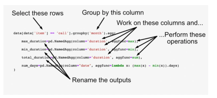
There were substantial changes to the Pandas aggregation function in May of 2017. Renaming of variables using dictionaries within the agg() function as in the diagram below is being deprecated/removed from Pandas – see notes.
 Aggregation of variables in a Pandas Dataframe using the agg() function. Note that in Pandas versions 0.20.1 onwards, the renaming of results needs to be done separately.
In older Pandas releases (< 0.20.1), renaming the newly calculated columns was possible through nested dictionaries, or by passing a list of functions for a column. Our final example calculates multiple values from the duration column and names the results appropriately. Note that the results have multi-indexed column headers.
Note this syntax will no longer work for new installations of Python Pandas.

Summary of Python Pandas Grouping
The groupby functionality in Pandas is well documented in the official docs and performs at speeds on a par (unless you have massive data and are picky with your milliseconds) with R’s data.table and dplyr libraries.
If you are interested in another example for practice, I used these same techniques to analyse weather data for this post, and I’ve put “how-to” instructions here.
There are plenty of resources online on this functionality, and I’d recommomend really conquering this syntax if you’re using Pandas in earnest at any point.
- DataQuest Tutorial on Data Analysis: https://www.dataquest.io/blog/pandas-tutorial-python-2/
- Chris Albon notes on Groups: https://chrisalbon.com/python/pandas_apply_operations_to_groups.html
- Greg Reda Pandas Tutorial: http://www.gregreda.com/2013/10/26/working-with-pandas-dataframes/