Householder transformation

Householder transformation

Wiki: Householder transformation is a linear transformation that reflect vector \(x\) about a hyperplane to obtain \(x^{\prime}\).

Please refer the these video1 and video2 for detailed deductions.

In order to obtain vector \(x^\prime\) which is the reflection of vector \(x\) with respect to the hyperplane of which the normal vector is denoted as \(u\), we follows the procedures below:

\[\text{Projection of vecotr x on u is: } \frac{\vec{x}\cdot\vec{u}}{\|\vec{u}\|^2}\vec{u}\\ \text{Let: }\vec{v}=\frac{\vec{u}}{\|\vec{u}\|},\text{we get the normalized normal vector}\\ \therefore \vec{x}^{\prime}=\vec{x}-2\frac{\vec{x}\cdot\vec{u}}{\|\vec{u}\|^2}\vec{u}=\vec{x}-2\vec{v}\vec{v}^T\vec{x}=(1-2\vec{v}\vec{v}^T)\vec{x} \]

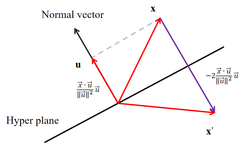
Here we define the following as the householder matrix:

\[H=1-2\vec{v}\vec{v}^T \]

And:

\[\vec{x}^{\prime}=H\vec{x} \]

Let's look into an example to see how householder transformation is related to QR decomposition.

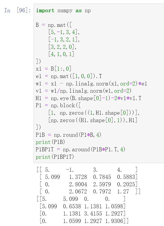
Consider the following matrix \(B\):

\[B = \begin{bmatrix}-1&-1&1\\1&3&3\\-1&-1&5\end{bmatrix}=\begin{bmatrix}x_1&x_2&x_3\end{bmatrix}\\ x_1=\begin{bmatrix}-1&1&-1\end{bmatrix}^T,x_2=\begin{bmatrix}-1&3&-1\end{bmatrix}^T,x_3=\begin{bmatrix}1&3&5\end{bmatrix}^T \]

So matrix \(B\) represents a space which is spanned by those column vectors.

We choose \(x_1\), and we imagine that after reflection, \(x_1\) is laid on the first basis vector \(e_1=\begin{bmatrix}1,0,\cdots,0\end{bmatrix}^T\) , which means that \(x_1^{\prime}=\|x_1\|e_1\). So we can easily obtain \(v_1\) (normalized normal vector), which is:

\[w_1=x_1-\|x_1\|e_1=\begin{bmatrix}-1\\1\\-1\end{bmatrix}-\sqrt{3}\begin{bmatrix}1\\0\\0\end{bmatrix}=\begin{bmatrix}-2.7321\\1.0000\\-1.0000\end{bmatrix}\\ v_1=\frac{w_1}{\|w_1\|}=\begin{bmatrix}-0.8881\\0.3251\\-0.3251\end{bmatrix} \]

Then the householder matrix for \(x_1\) is:

\[H_1= I-2vv^T=\begin{bmatrix}-0.5774 &0.5774&-0.5774\\0.5574&0.7887&0.2113\\-0.5774&0.2113&0.7887\end{bmatrix} \]

Therefore:

\[H_1B=\begin{bmatrix}-0.5774 &0.5774&-0.5774\\0.5574&0.7887&0.2113\\-0.5774&0.2113&0.7887\end{bmatrix}\begin{bmatrix}-1&-1&1\\1&3&3\\-1&-1&5\end{bmatrix}\\ =R_1=\begin{bmatrix}1.7321&2.8868&-1.7321\\0&1.5774&4.0000\\0&0.4226&4.0000\end{bmatrix} \]

And we also define:

\[Q_1=H_1=\begin{bmatrix}-0.5774 &0.5774&-0.5774\\0.5574&0.7887&0.2113\\-0.5774&0.2113&0.7887\end{bmatrix} \]

Note that after the reflection of \(x_1\), the resultant entries of first column of \(R_1\) is all zero below the diagonal. This is because the \(H_1\) linear operation rotate the whole space and results in that \(x_1\) is located on the first basis vector \(e_1\). And the values on the diagonal is its norm.

Since the \(H_1\) is perform on the whole matrix, which means that the other vectors besides \(x_1\) will also rotate. Once we finish \(H_1\), we can continue to perform \(H_2,H_3,\cdots\) etc.

For example, we choose the second column of \(R_1\). Since vector \(x_2\) may not be complely orthogonal to vector \(x_1^{\prime}\), which means vector \(x_2\) may have some projection part on \(x_1^{'}\) and this refers to the \((1,2)\) entry. But we can neglact this and only focus on those components that are perpendicular to \(x_1^{\prime}\). That's why we choose \(x_2\) to be:

\[x_2=\begin{bmatrix}0&1.5774&0.4226\end{bmatrix}^T \]

in which the \((1,2)\) entry is set to zero.

And following the same algorithm, we obtain:

\[H_2 = \begin{bmatrix}1.0000&0&0\\0&0.9659&0.2588\\0&0.2588&-0.9659\end{bmatrix}\\ H_2R_1=\begin{bmatrix}1.0000&0&0\\0&0.9659&0.2588\\0&0.2588&-0.9659\end{bmatrix}\begin{bmatrix}1.7321&2.8868&-1.7321\\0&1.5774&4.0000\\0&0.4226&4.0000\end{bmatrix}\\ =R_2=\begin{bmatrix}1.7321&2.8868&-1.7321\\0&1.6330&4.8990\\0&0&-2.8284\end{bmatrix}=R\\ Q_2=H_1H_2=\begin{bmatrix}-0.5774 &0.5774&-0.5774\\0.5574&0.7887&0.2113\\-0.5774&0.2113&0.7887\end{bmatrix}\begin{bmatrix}1.0000&0&0\\0&0.9659&0.2588\\0&0.2588&-0.9659\end{bmatrix}\\ =\begin{bmatrix}-0.5774&-0.4082&-0.7071\\0.5774&-0.8165&0\\-0.5774&-0.4082&0.7071\end{bmatrix}=Q \]

Take a close look at \(R_2\), it is not surprising that becomes an upper triangular matrix. Focus on the second column, as we metioned before, the \(H_2\) operation only makes the perpendicular part of \(x_2\) with respect to \(x_1^{\prime}\) rotates to the direction of the second basic vector \(e_2\). Therefore, if we just focus on the rows below the diagonal, we find that it is the same with that of \(x_1^{\prime}\) with the diagonal entry \((2,2)\) displaying the norm.

And the repetitive householder transformation operations finally leads to the QR decomposition. What a coincidence. Cool!

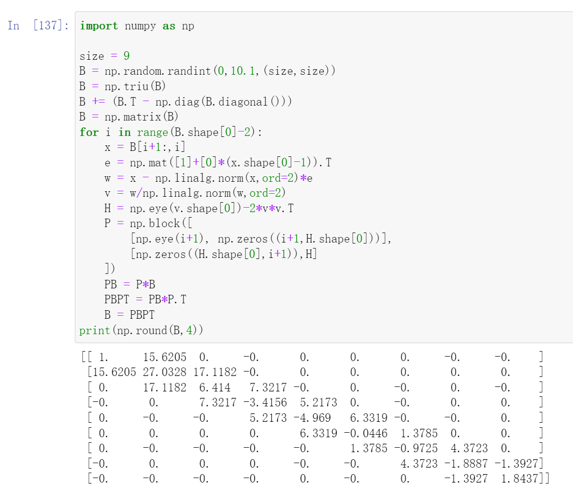
What would happen if we apply the householder transformations repetitively on a symmetric matrix from both sides? Like:

\[H_n\cdots H_2H_1BH_1^TH_2^T\cdots H_n^T \]

From our intuition, we might think that the combinition of \(H_1\) and \(H_1^T\) for example, will make the entries of the first column and first row to zeros except for the diagonal entry. And the repetitive procedures might result in a diagonal matrix. However, this does not actually hold as indicated by the test below:

Instead we will try to construct another householder matrix \(P\), and after applying \(P\) and its transpose \(P^T\) on matrix \(B\) repetitively, we end with a tridiagonal matrix.

For \(P_1\), it is represented by the following block matrix:

\[P_1=\begin{bmatrix}1&0\\0&H_1\end{bmatrix} \]

And \(H_1\) here is no longer a householder transformation matrix that applies to the first column vector. Instead, it applies to all the entries in the first column that are situated below the diagonal entry.

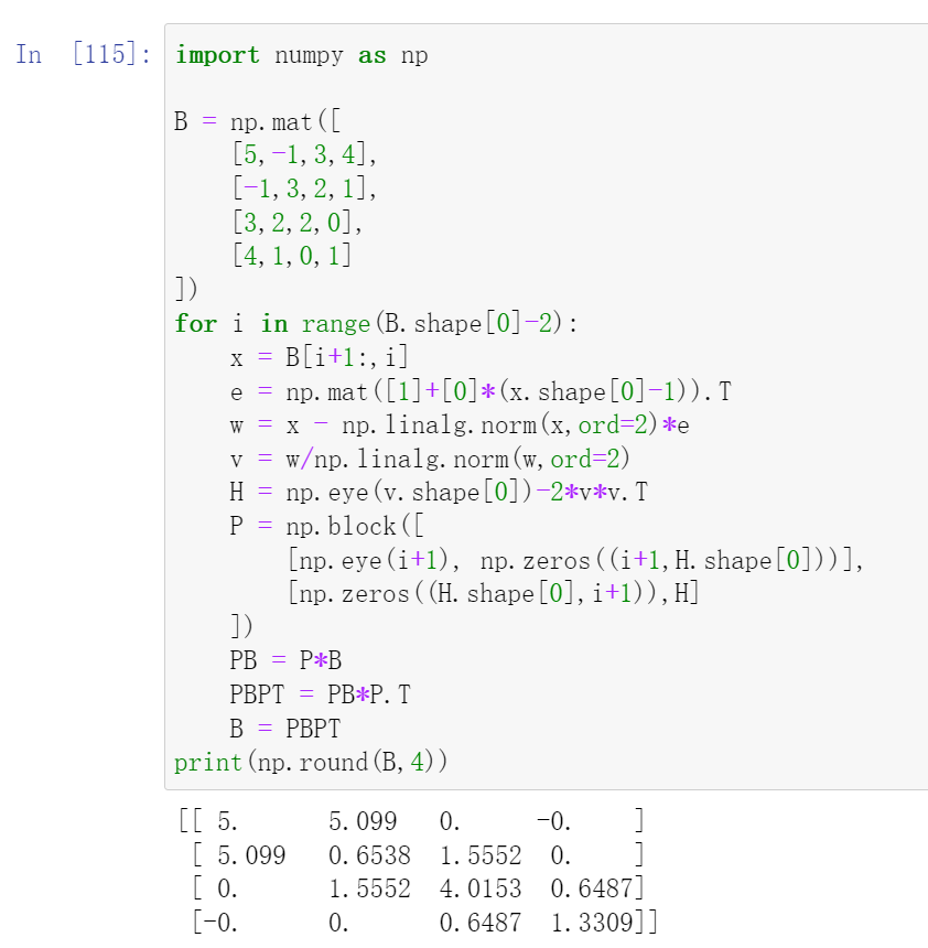
So the symmetric matrix \(B\) is:

\[\begin{bmatrix}5&-1&3&4\\-1&3&2&1\\3&2&2&0\\4&1&0&1\end{bmatrix} \]

Following the similar procedures, we have:

\[x_1=\begin{bmatrix}-1&3&4\end{bmatrix}^T\\ w_1 = x_1-\|x_1\|e_1=\begin{bmatrix}-1\\3\\4\end{bmatrix}-\sqrt{26}\begin{bmatrix}1\\0\\0\end{bmatrix}=\begin{bmatrix}-6.0990\\3.0000\\4.0000 \end{bmatrix}\\ v_1=\frac{w_1}{\|w_1\|}=\begin{bmatrix}-0.7733\\0.3804\\0.5072\end{bmatrix}\\H_1=I-2vv^T=\begin{bmatrix}-0.1961&0.5883&0.7845\\0.5883&0.7106&-0.3859\\0.7845&-0.3859&0.4855\end{bmatrix}\\ P_1 = \begin{bmatrix}1&0&0&0\\0&-0.1961&0.5883&0.7845\\0&0.5883&0.7106&-0.3859\\0&0.7845&-0.3859&0.4855\end{bmatrix}=\begin{bmatrix}1&0\\0&H_1\end{bmatrix}\\ \]

After we apply \(P_1\) to \(B\), we get all entries below the subdiagonal in the first column become zero. And by symmetry, when we continue to apply the transpose \(P_1^T\) rom right, we succeed to get all entries above the superdiagonal in the first row become zero. Take a close look at the following code:

And if we continue to do this, we will end up with a tridiagonal matrix：

For a more general case: