Audio Deep Learning Made Simple

https://towardsdatascience.com/audio-deep-learning-made-simple-part-1-state-of-the-art-techniques-da1d3dff2504

Although Computer Vision and NLP applications get most of the buzz, there are many groundbreaking use cases for deep learning with audio data that are transforming our daily lives. Over the next few articles, I aim to explore the fascinating world of audio deep learning.

Here’s a quick summary of the articles I am planning in the series. My goal throughout will be to understand not just how something works but why it works that way.

1. State-of-the-Art Techniques— this article (What is sound and how it is digitized. What problems is audio deep learning solving in our daily lives. What are Spectrograms and why they are all-important.)
2. Why Mel Spectrograms perform better (Processing audio data in Python. What are Mel Spectrograms and how to generate them)
3. Feature Optimization and Augmentation (Enhance Spectrograms features for optimal performance by hyper-parameter tuning and data augmentation)
4. Audio Classification (End-to-end example and architecture to classify ordinary sounds. Foundational application for a range of scenarios.)
5. Automatic Speech Recognition (Speech-to-Text algorithm and architecture, using CTC Loss and Decoding for aligning sequences.)
6. Beam Search (Algorithm commonly used by Speech-to-Text and NLP applications to enhance predictions)

In this first article, since this area may not be as familiar to people, I will introduce the topic and provide an overview of the deep learning landscape for audio applications. We will understand what audio is and how it is represented digitally. I will talk about the wide-ranging impact that audio applications have on our daily lives, and explore the architecture and model techniques that they use.

What is sound?

We all remember from school that a sound signal is produced by variations in air pressure. We can measure the intensity of the pressure variations and plot those measurements over time.

Sound signals often repeat at regular intervals so that each wave has the same shape. The height shows the intensity of the sound and is known as the amplitude.

Simple repeating signal showing Amplitude vs Time (by permission of Prof Mark Liberman)

The time taken for the signal to complete one full wave is the period. The number of waves made by the signal in one second is called the frequency. The frequency is the reciprocal of the period. The unit of frequency is Hertz.

The majority of sounds we encounter may not follow such simple and regular periodic patterns. But signals of different frequencies can be added together to create composite signals with more complex repeating patterns. All sounds that we hear, including our own human voice, consist of waveforms like these. For instance, this could be the sound of a musical instrument.

Musical waveform with a complex repeating signal (Source, by permission of Prof George Gibson)

The human ear is able to differentiate between different sounds based on the ‘quality’ of the sound which is also known as timbre.

How do we represent sound digitally?

To digitize a sound wave we must turn the signal into a series of numbers so that we can input it into our models. This is done by measuring the amplitude of the sound at fixed intervals of time.

Sample measurements at regular time intervals (Source)

Each such measurement is called a sample, and the sample rate is the number of samples per second. For instance, a common sampling rate is about 44,100 samples per second. That means that a 10-second music clip would have 441,000 samples!

Preparing audio data for a deep learning model

Till a few years ago, in the days before Deep Learning, machine learning applications of Computer Vision used to rely on traditional image processing techniques to do feature engineering. For instance, we would generate hand-crafted features using algorithms to detect corners, edges, and faces. With NLP applications as well, we would rely on techniques such as extracting N-grams and computing Term Frequency.

Similarly, audio machine learning applications used to depend on traditional digital signal processing techniques to extract features. For instance, to understand human speech, audio signals could be analyzed using phonetics concepts to extract elements like phonemes. All of this required a lot of domain-specific expertise to solve these problems and tune the system for better performance.

However, in recent years, as Deep Learning becomes more and more ubiquitous, it has seen tremendous success in handling audio as well. With deep learning, the traditional audio processing techniques are no longer needed, and we can rely on standard data preparation without requiring a lot of manual and custom generation of features.

What is more interesting is that, with deep learning, we don’t actually deal with audio data in its raw form. Instead, the common approach used is to convert the audio data into images and then use a standard CNN architecture to process those images! Really? Convert sound into pictures? That sounds like science fiction. 😄

The answer, of course, is fairly commonplace and mundane. This is done by generating Spectrograms from the audio. So first let’s learn what a Spectrum is, and use that to understand Spectrograms.

Spectrum

As we discussed earlier, signals of different frequencies can be added together to create composite signals, representing any sound that occurs in the real-world. This means that any signal consists of many distinct frequencies and can be expressed as the sum of those frequencies.

The Spectrum is the set of frequencies that are combined together to produce a signal. eg. the picture shows the spectrum of a piece of music.

The Spectrum plots all of the frequencies that are present in the signal along with the strength or amplitude of each frequency.

Spectrum showing the frequencies that make up a sound signal (Source, by permission of Prof Barry Truax)

The lowest frequency in a signal called the fundamental frequency. Frequencies that are whole number multiples of the fundamental frequency are known as harmonics.

For instance, if the fundamental frequency is 200 Hz, then its harmonic frequencies are 400 Hz, 600 Hz, and so on.

Time Domain vs Frequency Domain

The waveforms that we saw earlier showing Amplitude against Time are one way to represent a sound signal. Since the x-axis shows the range of time values of the signal, we are viewing the signal in the Time Domain.

The Spectrum is an alternate way to represent the same signal. It shows Amplitude against Frequency, and since the x-axis shows the range of frequency values of the signal, at a moment in time, we are viewing the signal in the Frequency Domain.

Time Domain and Frequency Domain (Source)

Spectrograms

Since a signal produces different sounds as it varies over time, its constituent frequencies also vary with time. In other words, its Spectrum varies with time.

A Spectrogram of a signal plots its Spectrum over time and is like a ‘photograph’ of the signal. It plots Time on the x-axis and Frequency on the y-axis. It is as though we took the Spectrum again and again at different instances in time, and then joined them all together into a single plot.

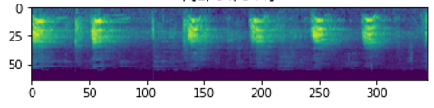
It uses different colors to indicate the Amplitude or strength of each frequency. The brighter the color the higher the energy of the signal. Each vertical ‘slice’ of the Spectrogram is essentially the Spectrum of the signal at that instant in time and shows how the signal strength is distributed in every frequency found in the signal at that instant.

In the example below, the first picture displays the signal in the Time domain ie. Amplitude vs Time. It gives us a sense of how loud or quiet a clip is at any point in time, but it gives us very little information about which frequencies are present.

Sound signal and its Spectrogram (Image by Author)

The second picture is the Spectrogram and displays the signal in the Frequency domain.

Generating Spectrograms

Spectrograms are produced using Fourier Transforms to decompose any signal into its constituent frequencies. If this makes you a little nervous because we have now forgotten all that we learned about Fourier Transforms during college, don’t worry 😄! We won’t actually need to recall all the mathematics, there are very convenient Python library functions that can generate spectrograms for us in a single step. We’ll see those in the next article.

Audio Deep Learning Models

Now that we understand what a Spectrogram is, we realize that it is an equivalent compact representation of an audio signal, somewhat like a ‘fingerprint’ of the signal. It is an elegant way to capture the essential features of audio data as an image.

Typical pipeline used by audio deep learning models (Image by Author)

So most deep learning audio applications use Spectrograms to represent audio. They usually follow a procedure like this:

• Start with raw audio data in the form of a wave file.
• Convert the audio data into its corresponding spectrogram.
• Optionally, use simple audio processing techniques to augment the spectrogram data. (Some augmentation or cleaning can also be done on the raw audio data before the spectrogram conversion)
• Now that we have image data, we can use standard CNN architectures to process them and extract feature maps that are an encoded representation of the spectrogram image.

The next step is to generate output predictions from this encoded representation, depending on the problem that you are trying to solve.

• For instance, for an audio classification problem, you would pass this through a Classifier usually consisting of some fully connected Linear layers.
• For a Speech-to-Text problem, you could pass it through some RNN layers to extract text sentences from this encoded representation.

Of course, we are skipping many details, and making some broad generalizations, but in this article, we are staying at a fairly high-level. In the following articles, we’ll go into a lot more specifics about all of these steps and the architectures that are used.

What problems does audio deep learning solve?

Audio data in day-to-day life can come in innumerable forms such as human speech, music, animal voices, and other natural sounds as well as man-made sounds from human activity such as cars and machinery.

Given the prevalence of sounds in our lives and the range of sound types, it is not surprising that there are a vast number of usage scenarios that require us to process and analyze audio. Now that deep learning has come of age, it can be applied to solve a number of use cases.

Audio Classification

This is one of the most common use cases and involves taking a sound and assigning it to one of several classes. For instance, the task could be to identify the type or source of the sound. eg. is this a car starting, is this a hammer, a whistle, or a dog barking.

Classification of Ordinary sounds (Image by Author)

Obviously, the possible applications are vast. This could be applied to detect the failure of machinery or equipment based on the sound that it produces, or in a surveillance system, to detect security break-ins.

Audio Separation and Segmentation

Audio Separation involves isolating a signal of interest from a mixture of signals so that it can then be used for further processing. For instance, you might want to separate out individual people’s voices from a lot of background noise, or the sound of the violin from the rest of the musical performance.

Separating individual speakers from a video (Source, by permission of Ariel Ephrat)

Audio Segmentation is used to highlight relevant sections from the audio stream. For instance, it could be used for diagnostic purposes to detect the different sounds of the human heart and detect anomalies.

Music Genre Classification and Tagging

With the popularity of music streaming services, another common application that most of us are familiar with is to identify and categorize music based on the audio. The content of the music is analyzed to figure out the genre to which it belongs. This is a multi-label classification problem because a given piece of music might fall under more than one genre. eg. rock, pop, jazz, salsa, instrumental as well as other facets such as ‘oldies’, ‘female vocalist’, ‘happy’, ‘party music’ and so on.

Music Genre Classification and Tagging (Image by Author)

Of course, in addition to the audio itself, there is metadata about the music such as singer, release date, composer, lyrics and so on which would be used to add a rich set of tags to music.

This can be used to index music collections according to their audio features, to provide music recommendations based on a user’s preferences, or for searching and retrieving a song that is similar to a song to which you are listening.

Music Generation and Music Transcription

We have seen a lot of news these days about deep learning being used to programmatically generate extremely authentic-looking pictures of faces and other scenes, as well as being able to write grammatically correct and intelligent letters or news articles.

Music Generation (Image by Author)

Similarly, we are now able to generate synthetic music that matches a particular genre, instrument, or even a given composer’s style.

In a way, Music Transcription applies this capability in reverse. It takes some acoustics and annotates it, to create a music sheet containing the musical notes that are present in the music.

Voice Recognition

Technically this is also a classification problem but deals with recognizing spoken sounds. It could be used to identify the gender of a speaker, or their name (eg. is this Bill Gates or Tom Hanks, or is this Ketan’s voice vs an intruder’s)

Voice Recognition for Intruder Detection (Image by Author)

We might want to detect human emotion and identify the mood of the person from the tone of their voice eg. is the person happy, sad, angry, or stressed.

We could apply this to animal voices to identify the type of animal that is producing a sound, or potentially to identify whether it is a gentle affectionate purring sound, a threatening bark, or a frightened yelp.

Speech to Text and Text to Speech

When dealing with human speech, we can go a step further, and not just recognize the speaker, but understand what they are saying. This involves extracting the words from the audio, in the language in which it is spoken and transcribing it into text sentences.

This is one of the most challenging applications because it deals not just with analyzing audio, but also with NLP and requires developing some basic language capability to decipher distinct words from the uttered sounds.

Speech to Text (Image by Author)

Conversely, with Speech Synthesis, one could go in the other direction and take written text and generate speech from it, using, for instance, an artificial voice for conversational agents.

Being able to understand human speech obviously enables a huge number of useful applications both in our business and personal lives, and we are only just beginning to scratch the surface.

The most well-known examples that have achieved widespread use are virtual assistants like Alexa, Siri, Cortana, and Google Home, which are consumer-friendly products built around this capability.

Conclusion

In this article, we have stayed at a fairly high-level and explored the breadth of audio applications, and covered the general techniques applied to solve those problems.

In the next article, we will go into more of the technical details of pre-processing audio data and generating spectrograms. We will take a look at the hyperparameters that are used to tune performance.

That will then prepare us for delving deeper into a couple of end-to-end examples, starting with the Classification of ordinary sounds and culminating with the much more challenging Automatic Speech Recognition, where we will also cover the fascinating CTC algorithm.

 

Audio File Formats and Python Libraries

Audio data for your deep learning models will usually start out as digital audio files. From listening to sound recordings and music, we all know that these files are stored in a variety of formats based on how the sound is compressed. Examples of these formats are .wav, .mp3, .wma, .aac, .flac and many more.

Python has some great libraries for audio processing. Librosa is one of the most popular and has an extensive set of features. scipy is also commonly used. If you are using Pytorch, it has a companion library called torchaudio that is tightly integrated with Pytorch. It doesn’t have as much functionality as Librosa, but it is built specifically for deep learning.

They all let you read audio files in different formats. The first step is to load the file. With librosa:

?

1 2 3 4 5

import librosa   # Load the audio file AUDIO_FILE = './audio.wav' samples, sample_rate = librosa.load(AUDIO_FILE, sr=None)

Or, you can also do the same thing using scipy:

from scipy.io import wavfile
sample_rate, samples = wavfile.read(AUDIO_FILE)

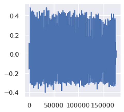
You can then visualize the sound wave:

import librosa.display
import matplotlib.pyplot as plt

# x-axis has been converted to time using our sample rate. 
# matplotlib plt.plot(y), would output the same figure, but with sample 
# number on the x-axis instead of seconds
plt.figure(figsize=(14, 5))
librosa.display.waveplot(samples, sr=sample_rate)

Visualize the sound wave (Image by Author)

And listen to it. If you are using a Jupyter notebook, you can play the audio directly in a cell.

from IPython.display import Audio
Audio(AUDIO_FILE)

Play audio in a notebook cell (Image by Author)

Audio Signal Data

As we saw in the previous article, audio data is obtained by sampling the sound wave at regular time intervals and measuring the intensity or amplitude of the wave at each sample. The metadata for that audio tells us the sampling rate which is the number of samples per second.

When that audio is saved in a file it is in a compressed format. When the file is loaded, it is decompressed and converted into a Numpy array. This array looks the same no matter which file format you started with.

In memory, audio is represented as a time series of numbers, representing the amplitude at each timestep. For instance, if the sample rate was 16800, a one-second clip of audio would have 16800 numbers. Since the measurements are taken at fixed intervals of time, the data contains only the amplitude numbers and not the time values. Given the sample rate, we can figure out at what time instant each amplitude number measurement was taken.

print ('Example shape ', samples.shape, 'Sample rate ', sample_rate, 'Data type', type(samples))
print (samples[22400:22420])

The bit-depth tells us how many possible values those amplitude measurements for each sample can take. For example, a bit-depth of 16 means that the amplitude number can be between 0 and 65535 (2 ¹⁶ — 1). The bit-depth influences the resolution of the audio measurement — the higher the bit-depth, the better the audio fidelity.

Bit-depth and sample-rate determine the audio resolution (Source)

Spectrograms

Deep learning models rarely take this raw audio directly as input. As we learned in Part 1, the common practice is to convert the audio into a spectrogram. The spectrogram is a concise ‘snapshot’ of an audio wave and since it is an image, it is well suited to being input to CNN-based architectures developed for handling images.

Spectrograms are generated from sound signals using Fourier Transforms. A Fourier Transform decomposes the signal into its constituent frequencies and displays the amplitude of each frequency present in the signal.

A Spectrogram chops up the duration of the sound signal into smaller time segments and then applies the Fourier Transform to each segment, to determine the frequencies contained in that segment. It then combines the Fourier Transforms for all those segments into a single plot.

It plots Frequency (y-axis) vs Time (x-axis) and uses different colors to indicate the Amplitude of each frequency. The brighter the color the higher the energy of the signal.

sgram = librosa.stft(samples)
librosa.display.specshow(sgram)

Simple Spectrogram (Image by Author)

Unfortunately, when we display this spectrogram there isn’t much information for us to see. What happened to all those colorful spectrograms we used to see in Science class?

This happens because of the way humans perceive sound. Most of what we are able to hear are concentrated in a narrow range of frequencies and amplitudes. Let’s explore that first so we can figure out how to produce those lovely spectrograms.

How do humans hear frequencies?

The way we hear frequencies in sound is known as ‘pitch’. It is a subjective impression of the frequency. So a high-pitched sound has a higher frequency than a low-pitched sound. Humans do not perceive frequencies linearly. We are more sensitive to differences between lower frequencies than higher frequencies.

For instance, if you listened to different pairs of sound as follows:

• 100Hz and 200Hz
• 1000Hz and 1100Hz
• 10000Hz and 10100 Hz

What is your perception of the “distance” between each pair of sounds? Are you able to tell each pair of sounds apart?

Even though in all cases, the actual frequency difference between each pair is exactly the same at 100 Hz, the pair at 100Hz and 200Hz will sound further apart than the pair at 1000Hz and 1100Hz. And you will hardly be able to distinguish between the pair at 10000Hz and 10100Hz.

However, this may seem less surprising if we realize that the 200Hz frequency is actually double the 100Hz, whereas the 10100Hz frequency is only 1% higher than the 10000Hz frequency.

This is how humans perceive frequencies. We hear them on a logarithmic scale rather than a linear scale. How do we account for this in our data?

Mel Scale

The Mel Scale was developed to take this into account by conducting experiments with a large number of listeners. It is a scale of pitches, such that each unit is judged by listeners to be equal in pitch distance from the next.

Mel Scale measures human perception of pitch (Source, by permission of Prof Barry Truax)

How do humans hear amplitudes?

The human perception of the amplitude of a sound is its loudness. And similar to frequency, we hear loudness logarithmically rather than linearly. We account for this using the Decibel scale.

Decibel Scale

On this scale, 0 dB is total silence. From there, measurement units increase exponentially. 10 dB is 10 times louder than 0 dB, 20 dB is 100 times louder and 30 dB is 1000 times louder. On this scale, a sound above 100 dB starts to become unbearably loud.

Decibel levels of common sounds (Adapted from Source)

We can see that, to deal with sound in a realistic manner, it is important for us to use a logarithmic scale via the Mel Scale and the Decibel Scale when dealing with Frequencies and Amplitudes in our data.

That is exactly what the Mel Spectrogram is intended to do.

Mel Spectrograms

A Mel Spectrogram makes two important changes relative to a regular Spectrogram that plots Frequency vs Time.

• It uses the Mel Scale instead of Frequency on the y-axis.
• It uses the Decibel Scale instead of Amplitude to indicate colors.

For deep learning models, we usually use this rather than a simple Spectrogram.

Let’s modify our Spectrogram code above to use the Mel Scale in place of Frequency.

# use the mel-scale instead of raw frequency
sgram_mag, _ = librosa.magphase(sgram)
mel_scale_sgram = librosa.feature.melspectrogram(S=sgram_mag, sr=sample_rate)
librosa.display.specshow(mel_scale_sgram)

Spectrogram using Mel Scale (Image by Author)

This is better than before, but most of the spectrogram is still dark and not carrying enough useful information. So let’s modify it to use the Decibel Scale instead of Amplitude.

# use the decibel scale to get the final Mel Spectrogram
mel_sgram = librosa.amplitude_to_db(mel_scale_sgram, ref=np.min)
librosa.display.specshow(mel_sgram, sr=sample_rate, x_axis='time', y_axis='mel')
plt.colorbar(format='%+2.0f dB')

Mel Spectrogram (Image by Author)

Finally! This is what we were really looking for 😃.

Conclusion

We have now seen how we pre-process audio data and prepare Mel Spectrograms. But before we can input them into deep learning models, we have to optimize them to obtain the best performance.

In the next article, we will look at how we can enhance the data for our models by tuning our Mel Spectrograms, as well as augmenting our audio data to help our models generalize to a wider range of inputs.

 

Spectrograms Optimization with Hyper-parameter tuning

In Part 2 we learned what a Mel Spectrogram is and how to create one using some convenient library functions. But to really get the best performance for our deep learning models, we should optimize the Mel Spectrograms for the problem that we’re trying to solve.

There are a number of hyper-parameters that we can use to tune how the Spectrogram is generated. For that, we need to understand a few concepts about how Spectrograms are constructed. (I’ll try to keep that as simple and intuitive as possible!)

Fast Fourier Transform (FFT)

One way to compute Fourier Transforms is by using a technique called DFT (Discrete Fourier Transform). The DFT is very expensive to compute, so in practice, the FFT (Fast Fourier Transform) algorithm is used, which is an efficient way to implement the DFT.

However, the FFT will give you the overall frequency components for the entire time series of the audio signal as a whole. It won’t tell you how those frequency components change over time within the audio signal. You will not be able to see, for example, that the first part of the audio had high frequencies while the second part had low frequencies, and so on.

Short-time Fourier Transform (STFT)

To get that more granular view and see the frequency variations over time, we use the STFT algorithm (Short-Time Fourier Transform). The STFT is another variant of the Fourier Transform that breaks up the audio signal into smaller sections by using a sliding time window. It takes the FFT on each section and then combines them. It is thus able to capture the variations of the frequency with time.

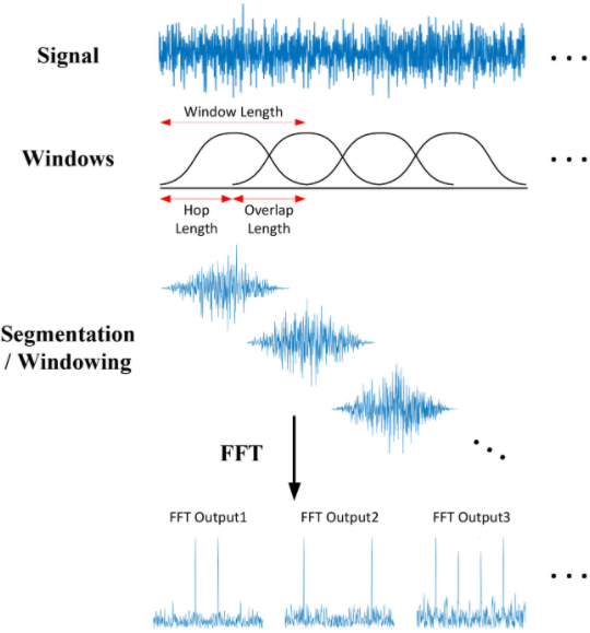
STFT slides an overlapping window along the signal and does a Fourier Transform on each segment (Source)

This splits the signal into sections along the Time axis. Secondly, it also splits the signal into sections along the Frequency axis. It takes the full range of frequencies and divides it up into equally spaced bands (in the Mel scale). Then, for each section of time, it calculates the Amplitude or energy for each frequency band.

#Spectrogram is a 2D numpy array
print(type(mel_sgram), mel_sgram.shape)
# <class 'numpy.ndarray'> (128, 134)

Let’s make this clear with an example. We have a 1-minute audio clip that contains frequencies between 0Hz and 10000 Hz (in the Mel scale). Let’s say that the Mel Spectrogram algorithm:

• Chooses windows such that it splits our audio signal into 20 time-sections.
• Decides to split our frequency range into 10 bands (ie. 0–1000Hz, 1000–2000Hz, … 9000–10000Hz).

The final output of the algorithm is a 2D Numpy array of shape (10, 20) where:

• Each of the 20 columns represents the FFT for one time-section.
• Each of the 10 rows represents Amplitude values for a frequency band.

Let’s take the first column, which is the FFT for the first time section. It has 10 rows.

• The first row is the Amplitude for the first frequency band between 0–1000 Hz.
• The second row is the Amplitude for the second frequency band between 1000–2000 Hz.
• … and so on.

Each column in the array becomes a ‘column’ in our Mel Spectrogram image.

Mel Spectrogram Hyperparameters

This gives us the hyperparameters for tuning our Mel Spectrogram. We’ll use the parameter names that Librosa uses. (Other libraries will have equivalent parameters)

Frequency Bands

• fmin — minimum frequency
• fmax — maximum frequency to display
• n_mels — number of frequency bands (ie. Mel bins). This is the height of the Spectrogram

Time Sections

• n_fft — window length for each time section
• hop_length — number of samples by which to slide the window at each step. Hence, the width of the Spectrogram is = Total number of samples / hop_length

You can adjust these hyperparameters based on the type of audio data that you have and the problem you’re solving.

MFCC (for Human Speech)

Mel Spectrograms work well for most audio deep learning applications. However, for problems dealing with human speech, like Automatic Speech Recognition, you might find that MFCC (Mel Frequency Cepstral Coefficients) sometimes work better.

These essentially take Mel Spectrograms and apply a couple of further processing steps. This selects a compressed representation of the frequency bands from the Mel Spectrogram that correspond to the most common frequencies at which humans speak.

import sklearn
import librosa
import librosa.display

# Load the audio file
samples, sample_rate = librosa.load(AUDIO_FILE, sr=None)
mfcc = librosa.feature.mfcc(samples, sr=sample_rate)

# Center MFCC coefficient dimensions to the mean and unit variance
mfcc = sklearn.preprocessing.scale(mfcc, axis=1)
librosa.display.specshow(mfcc, sr=sample_rate, x_axis='time')

print (f'MFCC is of type {type(mfcc)} with shape {mfcc.shape}')
# MFCC is of type <class 'numpy.ndarray'> with shape (20, 134)

MFCC generated from audio (Image by Author)

Above, we had seen that the Mel Spectrogram for this same audio had shape (128, 134), whereas the MFCC has shape (20, 134). The MFCC extracts a much smaller set of features from the audio that are the most relevant in capturing the essential quality of the sound.

Data Augmentation

A common technique to increase the diversity of your dataset, particularly when you don’t have enough data, is to augment your data artificially. We do this by modifying the existing data samples in small ways.

For instance, with images, we might do things like rotate the image slightly, crop or scale it, modify colors or lighting, or add some noise to the image. Since the semantics of the image haven’t changed materially, so the same target label from the original sample will still apply to the augmented sample. eg. if the image was labeled as a ‘cat’, the augmented image will also be a ‘cat’.

But, from the model’s point of view, it feels like a new data sample. This helps your model generalize to a larger range of image inputs.

Just like with images, there are several techniques to augment audio data as well. This augmentation can be done both on the raw audio before producing the spectrogram, or on the generated spectrogram. Augmenting the spectrogram usually produces better results.

Spectrogram Augmentation

The normal transforms you would use for an image don’t apply to spectrograms. For instance, a horizontal flip or a rotation would substantially alter the spectrogram and the sound that it represents.

Instead, we use a method known as SpecAugment where we block out sections of the spectrogram. There are two flavors:

• Frequency mask — randomly mask out a range of consecutive frequencies by adding horizontal bars on the spectrogram.
• Time mask — similar to frequency masks, except that we randomly block out ranges of time from the spectrogram by using vertical bars.

(Image by Author)

Raw Audio Augmentation

There are several options:

Time Shift — shift audio to the left or the right by a random amount.

• For sound such as traffic or sea waves which has no particular order, the audio could wrap around.

Augmentation by Time Shift (Image by Author)

• Alternately, for sounds such as human speech where the order does matter, the gaps can be filled with silence.

Pitch Shift — randomly modify the frequency of parts of the sound.

Augmentation by Pitch Shift (Image by Author)

Time Stretch — randomly slow down or speed up the sound.

Augmentation by Time Stretch (Image by Author)

Add Noise — add some random values to the sound.

Augmentation by Adding Noise (Image by Author)

Conclusion

We have now seen how we pre-process and prepare audio data for input to deep learning models. These approaches are commonly applied for a majority of audio applications.

We are now ready to explore some real deep learning applications and will cover an Audio Classification example in the next article, where we’ll see these techniques in action.

 

Audio Classification

Just like classifying hand-written digits using the MNIST dataset is considered a ‘Hello World”-type problem for Computer Vision, we can think of this application as the introductory problem for audio deep learning.

We will start with sound files, convert them into spectrograms, input them into a CNN plus Linear Classifier model, and produce predictions about the class to which the sound belongs.

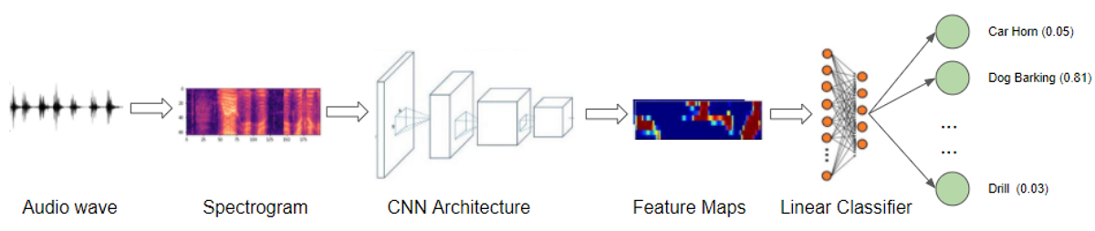
Audio Classification application (Image by Author)

There are many suitable datasets available for sounds of different types. These datasets contain a large number of audio samples, along with a class label for each sample that identifies what type of sound it is, based on the problem you are trying to address.

These class labels can often be obtained from some part of the filename of the audio sample or from the sub-folder name in which the file is located. Alternately the class labels are specified in a separate metadata file, usually in TXT, JSON, or CSV format.

Example problem — Classifying ordinary city sounds

For our demo, we will use the Urban Sound 8K dataset that consists of a corpus of ordinary sounds recorded from day-to-day city life. The sounds are taken from 10 classes such as drilling, dogs barking, and sirens. Each sound sample is labeled with the class to which it belongs.

After downloading the dataset, we see that it consists of two parts:

• Audio files in the ‘audio’ folder: It has 10 sub-folders named ‘fold1’ through ‘fold10’. Each sub-folder contains a number of ‘.wav’ audio samples eg. ‘fold1/103074–7–1–0.wav’
• Metadata in the ‘metadata’ folder: It has a file ‘UrbanSound8K.csv’ that contains information about each audio sample in the dataset such as its filename, its class label, the ‘fold’ sub-folder location, and so on. The class label is a numeric Class ID from 0–9 for each of the 10 classes. eg. the number 0 means air conditioner, 1 is a car horn, and so on.

The samples are around 4 seconds in length. Here’s what one sample looks like:

An audio sample of a drill (Image by Author)

Sample Rate, Number of Channels, Bits, and Audio Encoding

The recommendation of the dataset creators is to use the folds for doing 10-fold cross-validation to report metrics and evaluate the performance of your model. However, since our goal in this article is primarily as a demo of an audio deep learning example rather than to obtain the best metrics, we will ignore the folds and treat all the samples simply as one large dataset.

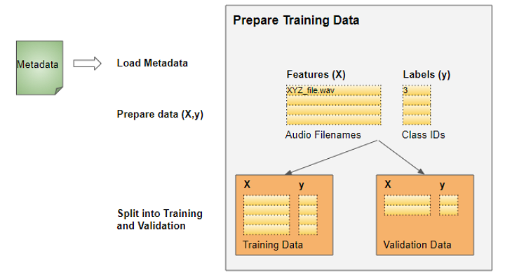
Prepare training data

As for most deep learning problems, we will follow these steps:

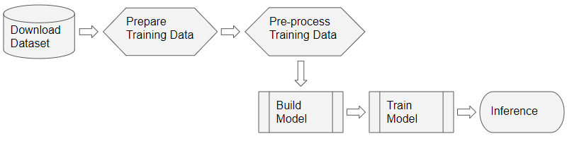
Deep Learning Workflow (Image by Author)

The training data for this problem will be fairly simple:

• The features (X) are the audio file paths
• The target labels (y) are the class names

Since the dataset has a metadata file that contains this information already, we can use that directly. The metadata contains information about each audio file.

Since it is a CSV file, we can use Pandas to read it. We can prepare the feature and label data from the metadata.

# ----------------------------
# Prepare training data from Metadata file
# ----------------------------
import pandas as pd
from pathlib import Path

download_path = Path.cwd()/'UrbanSound8K'

# Read metadata file
metadata_file = download_path/'metadata'/'UrbanSound8K.csv'
df = pd.read_csv(metadata_file)
df.head()

# Construct file path by concatenating fold and file name
df['relative_path'] = '/fold' + df['fold'].astype(str) + '/' + df['slice_file_name'].astype(str)

# Take relevant columns
df = df[['relative_path', 'classID']]
df.head()

This gives us the information we need for our training data.

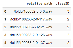
Training data with audio file paths and class IDs

Scan the audio file directory when metadata isn’t available

Having the metadata file made things easy for us. How would we prepare our data for datasets that do not contain a metadata file?

Many datasets consist of only audio files arranged in a folder structure from which class labels can be derived. To prepare our training data in this format, we would do the following:

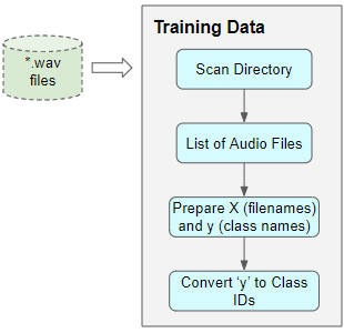
Preparing Training Data when metadata isn’t available (Image by Author)

• Scan the directory and prepare a list of all the audio file paths.
• Extract the class label from each file name, or from the name of the parent sub-folder
• Map each class name from text to a numeric class ID

With or without metadata, the result would be the same — features consisting of a list of audio file names and target labels consisting of class IDs.

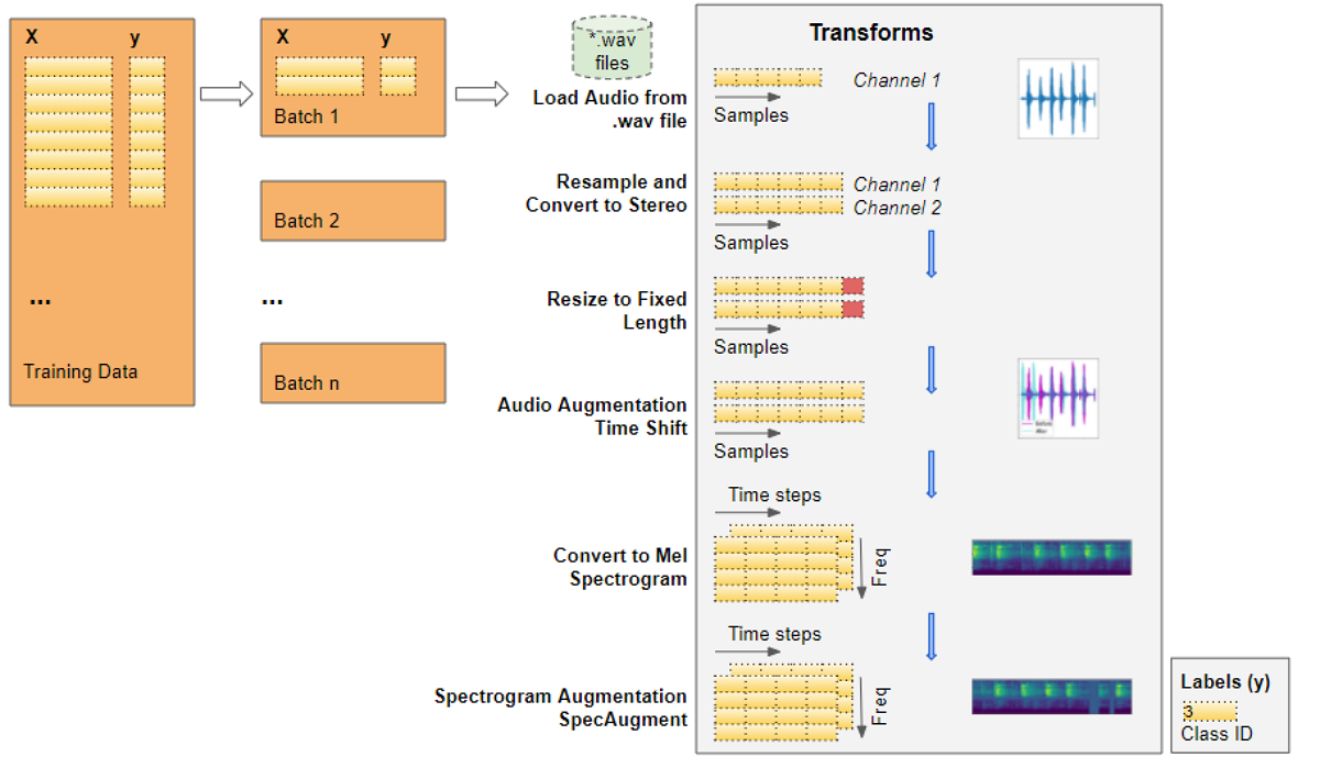
Audio Pre-processing: Define Transforms

This training data with audio file paths cannot be input directly into the model. We have to load the audio data from the file and process it so that it is in a format that the model expects.

This audio pre-processing will all be done dynamically at runtime when we will read and load the audio files. This approach is similar to what we would do with image files as well. Since audio data, like image data, can be fairly large and memory-intensive, we don’t want to read the entire dataset into memory all at once, ahead of time. So we keep only the audio file names (or image file names) in our training data.

Then, at runtime, as we train the model one batch at a time, we will load the audio data for that batch and process it by applying a series of transforms to the audio. That way we keep audio data for only one batch in memory at a time.

With image data, we might have a pipeline of transforms where we first read the image file as pixels and load it. Then we might apply some image processing steps to reshape and resize the data, crop them to a fixed size and convert them into grayscale from RGB. We might also apply some image augmentation steps like rotation, flips, and so on.

The processing for audio data is very similar. Right now we’re only defining the functions, they will be run a little later when we feed data to the model during training.

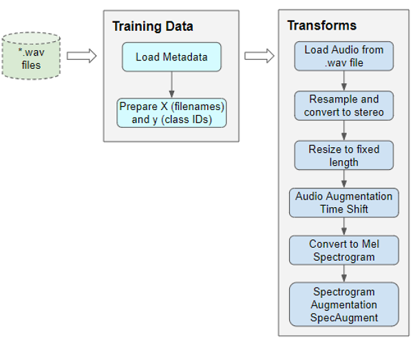
Pre-processing the training data for input to our model (Image by Author)

Read audio from a file

The first thing we need is to read and load the audio file in “.wav” format. Since we are using Pytorch for this example, the implementation below uses torchaudio for the audio processing, but librosa will work just as well.

import math, random
import torch
import torchaudio
from torchaudio import transforms
from IPython.display import Audio

class AudioUtil():
  # ----------------------------
  # Load an audio file. Return the signal as a tensor and the sample rate
  # ----------------------------
  @staticmethod
  def open(audio_file):
    sig, sr = torchaudio.load(audio_file)
    return (sig, sr)

Audio wave loaded from a file (Image by Author)

Convert to two channels

Some of the sound files are mono (ie. 1 audio channel) while most of them are stereo (ie. 2 audio channels). Since our model expects all items to have the same dimensions, we will convert the mono files to stereo, by duplicating the first channel to the second.

  # ----------------------------
  # Convert the given audio to the desired number of channels
  # ----------------------------
  @staticmethod
  def rechannel(aud, new_channel):
    sig, sr = aud

    if (sig.shape[0] == new_channel):
      # Nothing to do
      return aud

    if (new_channel == 1):
      # Convert from stereo to mono by selecting only the first channel
      resig = sig[:1, :]
    else:
      # Convert from mono to stereo by duplicating the first channel
      resig = torch.cat([sig, sig])

    return ((resig, sr))

Standardize sampling rate

Some of the sound files are sampled at a sample rate of 48000Hz, while most are sampled at a rate of 44100Hz. This means that 1 second of audio will have an array size of 48000 for some sound files, while it will have a smaller array size of 44100 for the others. Once again, we must standardize and convert all audio to the same sampling rate so that all arrays have the same dimensions.

  # ----------------------------
  # Since Resample applies to a single channel, we resample one channel at a time
  # ----------------------------
  @staticmethod
  def resample(aud, newsr):
    sig, sr = aud

    if (sr == newsr):
      # Nothing to do
      return aud

    num_channels = sig.shape[0]
    # Resample first channel
    resig = torchaudio.transforms.Resample(sr, newsr)(sig[:1,:])
    if (num_channels > 1):
      # Resample the second channel and merge both channels
      retwo = torchaudio.transforms.Resample(sr, newsr)(sig[1:,:])
      resig = torch.cat([resig, retwo])

    return ((resig, newsr))

Resize to the same length

We then resize all the audio samples to have the same length by either extending its duration by padding it with silence, or by truncating it. We add that method to our AudioUtil class.

  # ----------------------------
  # Pad (or truncate) the signal to a fixed length 'max_ms' in milliseconds
  # ----------------------------
  @staticmethod
  def pad_trunc(aud, max_ms):
    sig, sr = aud
    num_rows, sig_len = sig.shape
    max_len = sr//1000 * max_ms

    if (sig_len > max_len):
      # Truncate the signal to the given length
      sig = sig[:,:max_len]

    elif (sig_len < max_len):
      # Length of padding to add at the beginning and end of the signal
      pad_begin_len = random.randint(0, max_len - sig_len)
      pad_end_len = max_len - sig_len - pad_begin_len

      # Pad with 0s
      pad_begin = torch.zeros((num_rows, pad_begin_len))
      pad_end = torch.zeros((num_rows, pad_end_len))

      sig = torch.cat((pad_begin, sig, pad_end), 1)
      
    return (sig, sr)

Data Augmentation: Time Shift

Next, we can do data augmentation on the raw audio signal by applying a Time Shift to shift the audio to the left or the right by a random amount. I go into a lot more detail about this and other data augmentation techniques in this article.

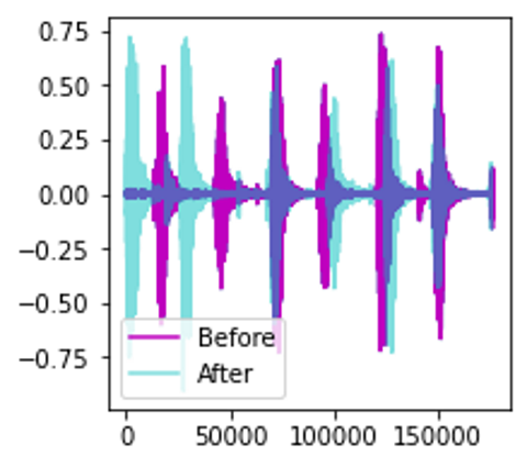
Time Shift of the audio wave (Image by Author)

  # ----------------------------
  # Shifts the signal to the left or right by some percent. Values at the end
  # are 'wrapped around' to the start of the transformed signal.
  # ----------------------------
  @staticmethod
  def time_shift(aud, shift_limit):
    sig,sr = aud
    _, sig_len = sig.shape
    shift_amt = int(random.random() * shift_limit * sig_len)
    return (sig.roll(shift_amt), sr)

Mel Spectrogram

We then convert the augmented audio to a Mel Spectrogram. They capture the essential features of the audio and are often the most suitable way to input audio data into deep learning models. To get more background about this, you might want to read my articles (here and here) which explain in simple words what a Mel Spectrogram is, why they are crucial for audio deep learning, as well as how they are generated and how to tune them for getting the best performance from your models.

  # ----------------------------
  # Generate a Spectrogram
  # ----------------------------
  @staticmethod
  def spectro_gram(aud, n_mels=64, n_fft=1024, hop_len=None):
    sig,sr = aud
    top_db = 80

    # spec has shape [channel, n_mels, time], where channel is mono, stereo etc
    spec = transforms.MelSpectrogram(sr, n_fft=n_fft, hop_length=hop_len, n_mels=n_mels)(sig)

    # Convert to decibels
    spec = transforms.AmplitudeToDB(top_db=top_db)(spec)
    return (spec)

Mel Spectrogram of an audio wave (Image by Author)

Data Augmentation: Time and Frequency Masking

Now we can do another round of augmentation, this time on the Mel Spectrogram rather than on the raw audio. We will use a technique called SpecAugment that uses these two methods:

• Frequency mask — randomly mask out a range of consecutive frequencies by adding horizontal bars on the spectrogram.
• Time mask — similar to frequency masks, except that we randomly block out ranges of time from the spectrogram by using vertical bars.

  # ----------------------------
  # Augment the Spectrogram by masking out some sections of it in both the frequency
  # dimension (ie. horizontal bars) and the time dimension (vertical bars) to prevent
  # overfitting and to help the model generalise better. The masked sections are
  # replaced with the mean value.
  # ----------------------------
  @staticmethod
  def spectro_augment(spec, max_mask_pct=0.1, n_freq_masks=1, n_time_masks=1):
    _, n_mels, n_steps = spec.shape
    mask_value = spec.mean()
    aug_spec = spec

    freq_mask_param = max_mask_pct * n_mels
    for _ in range(n_freq_masks):
      aug_spec = transforms.FrequencyMasking(freq_mask_param)(aug_spec, mask_value)

    time_mask_param = max_mask_pct * n_steps
    for _ in range(n_time_masks):
      aug_spec = transforms.TimeMasking(time_mask_param)(aug_spec, mask_value)

    return aug_spec

Mel Spectrogram after SpecAugment. Notice the horizontal and vertical mask bands (Image by Author)

Define Custom Data Loader

Now that we have defined all the pre-processing transform functions we will define a custom Pytorch Dataset object.

To feed your data to a model with Pytorch, we need two objects:

• A custom Dataset object that uses all the audio transforms to pre-process an audio file and prepares one data item at a time.
• A built-in DataLoader object that uses the Dataset object to fetch individual data items and packages them into a batch of data.

from torch.utils.data import DataLoader, Dataset, random_split
import torchaudio

# ----------------------------
# Sound Dataset
# ----------------------------
class SoundDS(Dataset):
  def __init__(self, df, data_path):
    self.df = df
    self.data_path = str(data_path)
    self.duration = 4000
    self.sr = 44100
    self.channel = 2
    self.shift_pct = 0.4
            
  # ----------------------------
  # Number of items in dataset
  # ----------------------------
  def __len__(self):
    return len(self.df)    
    
  # ----------------------------
  # Get i'th item in dataset
  # ----------------------------
  def __getitem__(self, idx):
    # Absolute file path of the audio file - concatenate the audio directory with
    # the relative path
    audio_file = self.data_path + self.df.loc[idx, 'relative_path']
    # Get the Class ID
    class_id = self.df.loc[idx, 'classID']

    aud = AudioUtil.open(audio_file)
    # Some sounds have a higher sample rate, or fewer channels compared to the
    # majority. So make all sounds have the same number of channels and same 
    # sample rate. Unless the sample rate is the same, the pad_trunc will still
    # result in arrays of different lengths, even though the sound duration is
    # the same.
    reaud = AudioUtil.resample(aud, self.sr)
    rechan = AudioUtil.rechannel(reaud, self.channel)

    dur_aud = AudioUtil.pad_trunc(rechan, self.duration)
    shift_aud = AudioUtil.time_shift(dur_aud, self.shift_pct)
    sgram = AudioUtil.spectro_gram(shift_aud, n_mels=64, n_fft=1024, hop_len=None)
    aug_sgram = AudioUtil.spectro_augment(sgram, max_mask_pct=0.1, n_freq_masks=2, n_time_masks=2)

    return aug_sgram, class_id

Prepare Batches of Data with the Data Loader

All of the functions we need to input our data to the model have now been defined.

We use our custom Dataset to load the Features and Labels from our Pandas dataframe and split that data randomly in an 80:20 ratio into training and validation sets. We then use them to create our training and validation Data Loaders.

Split our data for training and validation (Image by Author)

from torch.utils.data import random_split

myds = SoundDS(df, data_path)

# Random split of 80:20 between training and validation
num_items = len(myds)
num_train = round(num_items * 0.8)
num_val = num_items - num_train
train_ds, val_ds = random_split(myds, [num_train, num_val])

# Create training and validation data loaders
train_dl = torch.utils.data.DataLoader(train_ds, batch_size=16, shuffle=True)
val_dl = torch.utils.data.DataLoader(val_ds, batch_size=16, shuffle=False)

When we start training, the Data Loader will randomly fetch one batch of input Features containing the list of audio file names and run the pre-processing audio transforms on each audio file. It will also fetch a batch of the corresponding target Labels containing the class IDs. Thus it will output one batch of training data at a time, which can directly be fed as input to our deep learning model.

Data Loader applies transforms and prepares one batch of data at a time (Image by Author)

Let’s walk through the steps as our data gets transformed, starting with an audio file:

• The audio from the file gets loaded into a Numpy array of shape (num_channels, num_samples). Most of the audio is sampled at 44.1kHz and is about 4 seconds in duration, resulting in 44,100 * 4 = 176,400 samples. If the audio has 1 channel, the shape of the array will be (1, 176,400). Similarly, audio of 4 seconds duration with 2 channels and sampled at 48kHz will have 192,000 samples and a shape of (2, 192,000).
• Since the channels and sampling rates of each audio are different, the next two transforms resample the audio to a standard 44.1kHz and to a standard 2 channels.
• Since some audio clips might be more or less than 4 seconds, we also standardize the audio duration to a fixed length of 4 seconds. Now arrays for all items have the same shape of (2, 176,400)
• The Time Shift data augmentation now randomly shifts each audio sample forward or backward. The shapes are unchanged.
• The augmented audio is now converted into a Mel Spectrogram, resulting in a shape of (num_channels, Mel freq_bands, time_steps) = (2, 64, 344)
• The SpecAugment data augmentation now randomly applies Time and Frequency Masks to the Mel Spectrograms. The shapes are unchanged.

Thus, each batch will have two tensors, one for the X feature data containing the Mel Spectrograms and the other for the y target labels containing numeric Class IDs. The batches are picked randomly from the training data for each training epoch.

Each batch has a shape of (batch_sz, num_channels, Mel freq_bands, time_steps)

A batch of (X, y) data

We can visualize one item from the batch. We see the Mel Spectrogram with vertical and horizontal stripes showing the Frequency and Time Masking data augmentation.

The data is now ready for input to the model.

Create Model

The data processing steps that we just did are the most unique aspects of our audio classification problem. From here on, the model and training procedure are quite similar to what is commonly used in a standard image classification problem and are not specific to audio deep learning.

Since our data now consists of Spectrogram images, we build a CNN classification architecture to process them. It has four convolutional blocks which generate the feature maps. That data is then reshaped into the format we need so it can be input into the linear classifier layer, which finally outputs the predictions for the 10 classes.

The model takes a batch of pre-processed data and outputs class predictions (Image by Author)

A few more details about how the model processes a batch of data:

• A batch of images is input to the model with shape (batch_sz, num_channels, Mel freq_bands, time_steps) ie. (16, 2, 64, 344).
• Each CNN layer applies its filters to step up the image depth ie. number of channels. The image width and height are reduced as the kernels and strides are applied. Finally, after passing through the four CNN layers, we get the output feature maps ie. (16, 64, 4, 22).
• This gets pooled and flattened to a shape of (16, 64) and then input to the Linear layer.
• The Linear layer outputs one prediction score per class ie. (16, 10)

import torch.nn.functional as F
from torch.nn import init

# ----------------------------
# Audio Classification Model
# ----------------------------
class AudioClassifier (nn.Module):
    # ----------------------------
    # Build the model architecture
    # ----------------------------
    def __init__(self):
        super().__init__()
        conv_layers = []

        # First Convolution Block with Relu and Batch Norm. Use Kaiming Initialization
        self.conv1 = nn.Conv2d(2, 8, kernel_size=(5, 5), stride=(2, 2), padding=(2, 2))
        self.relu1 = nn.ReLU()
        self.bn1 = nn.BatchNorm2d(8)
        init.kaiming_normal_(self.conv1.weight, a=0.1)
        self.conv1.bias.data.zero_()
        conv_layers += [self.conv1, self.relu1, self.bn1]

        # Second Convolution Block
        self.conv2 = nn.Conv2d(8, 16, kernel_size=(3, 3), stride=(2, 2), padding=(1, 1))
        self.relu2 = nn.ReLU()
        self.bn2 = nn.BatchNorm2d(16)
        init.kaiming_normal_(self.conv2.weight, a=0.1)
        self.conv2.bias.data.zero_()
        conv_layers += [self.conv2, self.relu2, self.bn2]

        # Second Convolution Block
        self.conv3 = nn.Conv2d(16, 32, kernel_size=(3, 3), stride=(2, 2), padding=(1, 1))
        self.relu3 = nn.ReLU()
        self.bn3 = nn.BatchNorm2d(32)
        init.kaiming_normal_(self.conv3.weight, a=0.1)
        self.conv3.bias.data.zero_()
        conv_layers += [self.conv3, self.relu3, self.bn3]

        # Second Convolution Block
        self.conv4 = nn.Conv2d(32, 64, kernel_size=(3, 3), stride=(2, 2), padding=(1, 1))
        self.relu4 = nn.ReLU()
        self.bn4 = nn.BatchNorm2d(64)
        init.kaiming_normal_(self.conv4.weight, a=0.1)
        self.conv4.bias.data.zero_()
        conv_layers += [self.conv4, self.relu4, self.bn4]

        # Linear Classifier
        self.ap = nn.AdaptiveAvgPool2d(output_size=1)
        self.lin = nn.Linear(in_features=64, out_features=10)

        # Wrap the Convolutional Blocks
        self.conv = nn.Sequential(*conv_layers)
 
    # ----------------------------
    # Forward pass computations
    # ----------------------------
    def forward(self, x):
        # Run the convolutional blocks
        x = self.conv(x)

        # Adaptive pool and flatten for input to linear layer
        x = self.ap(x)
        x = x.view(x.shape[0], -1)

        # Linear layer
        x = self.lin(x)

        # Final output
        return x

# Create the model and put it on the GPU if available
myModel = AudioClassifier()
device = torch.device("cuda:0" if torch.cuda.is_available() else "cpu")
myModel = myModel.to(device)
# Check that it is on Cuda
next(myModel.parameters()).device

Training

We are now ready to create the training loop to train the model.

We define the functions for the optimizer, loss, and scheduler to dynamically vary our learning rate as training progresses, which usually allows training to converge in fewer epochs.

We train the model for several epochs, processing a batch of data in each iteration. We keep track of a simple accuracy metric which measures the percentage of correct predictions.

# ----------------------------
# Training Loop
# ----------------------------
def training(model, train_dl, num_epochs):
  # Loss Function, Optimizer and Scheduler
  criterion = nn.CrossEntropyLoss()
  optimizer = torch.optim.Adam(model.parameters(),lr=0.001)
  scheduler = torch.optim.lr_scheduler.OneCycleLR(optimizer, max_lr=0.001,
                                                steps_per_epoch=int(len(train_dl)),
                                                epochs=num_epochs,
                                                anneal_strategy='linear')

  # Repeat for each epoch
  for epoch in range(num_epochs):
    running_loss = 0.0
    correct_prediction = 0
    total_prediction = 0

    # Repeat for each batch in the training set
    for i, data in enumerate(train_dl):
        # Get the input features and target labels, and put them on the GPU
        inputs, labels = data[0].to(device), data[1].to(device)

        # Normalize the inputs
        inputs_m, inputs_s = inputs.mean(), inputs.std()
        inputs = (inputs - inputs_m) / inputs_s

        # Zero the parameter gradients
        optimizer.zero_grad()

        # forward + backward + optimize
        outputs = model(inputs)
        loss = criterion(outputs, labels)
        loss.backward()
        optimizer.step()
        scheduler.step()

        # Keep stats for Loss and Accuracy
        running_loss += loss.item()

        # Get the predicted class with the highest score
        _, prediction = torch.max(outputs,1)
        # Count of predictions that matched the target label
        correct_prediction += (prediction == labels).sum().item()
        total_prediction += prediction.shape[0]

        #if i % 10 == 0:    # print every 10 mini-batches
        #    print('[%d, %5d] loss: %.3f' % (epoch + 1, i + 1, running_loss / 10))
    
    # Print stats at the end of the epoch
    num_batches = len(train_dl)
    avg_loss = running_loss / num_batches
    acc = correct_prediction/total_prediction
    print(f'Epoch: {epoch}, Loss: {avg_loss:.2f}, Accuracy: {acc:.2f}')

  print('Finished Training')
  
num_epochs=2   # Just for demo, adjust this higher.
training(myModel, train_dl, num_epochs)

Inference

Ordinarily, as part of the training loop, we would also evaluate our metrics on the validation data. We would then do inference on unseen data, perhaps by keeping aside a test dataset from the original data. However, for the purposes of this demo, we will use the validation data for this purpose.

We run an inference loop taking care to disable the gradient updates. The forward pass is executed with the model to get predictions, but we do not need to backpropagate or run the optimizer.

# ----------------------------
# Inference
# ----------------------------
def inference (model, val_dl):
  correct_prediction = 0
  total_prediction = 0

  # Disable gradient updates
  with torch.no_grad():
    for data in val_dl:
      # Get the input features and target labels, and put them on the GPU
      inputs, labels = data[0].to(device), data[1].to(device)

      # Normalize the inputs
      inputs_m, inputs_s = inputs.mean(), inputs.std()
      inputs = (inputs - inputs_m) / inputs_s

      # Get predictions
      outputs = model(inputs)

      # Get the predicted class with the highest score
      _, prediction = torch.max(outputs,1)
      # Count of predictions that matched the target label
      correct_prediction += (prediction == labels).sum().item()
      total_prediction += prediction.shape[0]
    
  acc = correct_prediction/total_prediction
  print(f'Accuracy: {acc:.2f}, Total items: {total_prediction}')

# Run inference on trained model with the validation set
inference(myModel, val_dl)

Conclusion

We have now seen an end-to-end example of sound classification which is one of the most foundational problems in audio deep learning. Not only is this used in a wide range of applications, but many of the concepts and techniques that we covered here will be relevant to more complicated audio problems such as automatic speech recognition where we start with human speech, understand what people are saying, and convert it to text.

 

Speech-to-Text

As we can imagine, human speech is fundamental to our daily personal and business lives, and Speech-to-Text functionality has a huge number of applications. One could use it to transcribe the content of customer support or sales calls, for voice-oriented chatbots, or to note down the content of meetings and other discussions.

Basic audio data consists of sounds and noises. Human speech is a special case of that. So concepts that I have talked about in my articles, such as how we digitize sound, process audio data, and why we convert audio to spectrograms, also apply to understanding speech. However, speech is more complicated because it encodes language.

Problems like audio classification start with a sound clip and predict which class that sound belongs to, from a given set of classes. For Speech-to-Text problems, your training data consists of:

• Input features (X): audio clips of spoken words
• Target labels (y): a text transcript of what was spoken

Automatic Speech Recognition uses audio waves as input features and the text transcript as target labels (Image by Author)

The goal of the model is to learn how to take the input audio and predict the text content of the words and sentences that were uttered.

Data pre-processing

In the sound classification article, I explain, step-by-step, the transforms that are used to process audio data for deep learning models. With human speech as well we follow a similar approach. There are several Python libraries that provide the functionality to do this, with librosa being one of the most popular.

Transforming raw audio waves to spectrogram images for input to a deep learning model (Image by Author)

Load Audio Files

• Start with input data that consists of audio files of the spoken speech in an audio format such as “.wav” or “.mp3”.
• Read the audio data from the file and load it into a 2D Numpy array. This array consists of a sequence of numbers, each representing a measurement of the intensity or amplitude of the sound at a particular moment in time. The number of such measurements is determined by the sampling rate. For instance, if the sampling rate was 44.1kHz, the Numpy array will have a single row of 44,100 numbers for 1 second of audio.
• Audio can have one or two channels, known as mono or stereo, in common parlance. With two-channel audio, we would have another similar sequence of amplitude numbers for the second channel. In other words, our Numpy array will be 3D, with a depth of 2.

Convert to uniform dimensions: sample rate, channels, and duration

• We might have a lot of variation in our audio data items. Clips might be sampled at different rates, or have a different number of channels. The clips will most likely have different durations. As explained above this means that the dimensions of each audio item will be different.
• Since our deep learning models expect all our input items to have a similar size, we now perform some data cleaning steps to standardize the dimensions of our audio data. We resample the audio so that every item has the same sampling rate. We convert all items to the same number of channels. All items also have to be converted to the same audio duration. This involves padding the shorter sequences or truncating the longer sequences.
• If the quality of the audio was poor, we might enhance it by applying a noise-removal algorithm to eliminate background noise so that we can focus on the spoken audio.

Data Augmentation of raw audio

• We could apply some data augmentation techniques to add more variety to our input data and help the model learn to generalize to a wider range of inputs. We could Time Shift our audio left or right randomly by a small percentage, or change the Pitch or the Speed of the audio by a small amount.

Mel Spectrograms

• This raw audio is now converted to Mel Spectrograms. A Spectrogram captures the nature of the audio as an image by decomposing it into the set of frequencies that are included in it.

MFCC

• For human speech, in particular, it sometimes helps to take one additional step and convert the Mel Spectrogram into MFCC (Mel Frequency Cepstral Coefficients). MFCCs produce a compressed representation of the Mel Spectrogram by extracting only the most essential frequency coefficients, which correspond to the frequency ranges at which humans speak.

Data Augmentation of Spectrograms

• We can now apply another data augmentation step on the Mel Spectrogram images, using a technique known as SpecAugment. This involves Frequency and Time Masking that randomly masks out either vertical (ie. Time Mask) or horizontal (ie. Frequency Mask) bands of information from the Spectrogram. NB: I’m not sure whether this can also be applied to MFCCs and whether that produces good results.

We have now transformed our original raw audio file into Mel Spectrogram (or MFCC) images after data cleaning and augmentation.

We also need to prepare the target labels from the transcript. This is simply regular text consisting of sentences of words, so we build a vocabulary from each character in the transcript and convert them into character IDs.

This gives us our input features and our target labels. This data is ready to be input into our deep learning model.

Architecture

There are many variations of deep learning architecture for ASR. Two commonly used approaches are:

• A CNN (Convolutional Neural Network) plus RNN-based (Recurrent Neural Network) architecture that uses the CTC Loss algorithm to demarcate each character of the words in the speech. eg. Baidu’s Deep Speech model.
• An RNN-based sequence-to-sequence network that treats each ‘slice’ of the spectrogram as one element in a sequence eg. Google’s Listen Attend Spell (LAS) model.

Let’s pick the first approach above and explore in more detail how that works. At a high level, the model consists of these blocks:

• A regular convolutional network consisting of a few Residual CNN layers that process the input spectrogram images and output feature maps of those images.

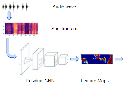
Spectrograms are processed by a convolutional network to produce feature maps (Image by Author)

• A regular recurrent network consisting of a few Bidirectional LSTM layers that process the feature maps as a series of distinct timesteps or ‘frames’ that correspond to our desired sequence of output characters. (An LSTM is a very commonly used type of recurrent layer, whose full form is Long Short Term Memory). In other words, it takes the feature maps which are a continuous representation of the audio, and converts them into a discrete representation.

Recurrent network processes frames from the feature maps (Image by Author)

• A linear layer with softmax that uses the LSTM outputs to produce character probabilities for each timestep of the output.

Linear layer generates character probabilities for each timestep (Image by Author)

• We also have linear layers that sit between the convolution and recurrent networks and help to reshape the outputs of one network to the inputs of the other.

So our model takes the Spectrogram images and outputs character probabilities for each timestep or ‘frame’ in that Spectrogram.

Align the sequences

If you think about this a little bit, you’ll realize that there is still a major missing piece in our puzzle. Our eventual goal is to map those timesteps or ‘frames’ to individual characters in our target transcript.

The model decodes the character probabilities to produce the final output (Image by Author)

But for a particular spectrogram, how do we know how many frames there should be? How do we know exactly where the boundaries of each frame are? How do we align the audio with each character in the text transcript?

On the left is the alignment we need. But how do we get it?? (Image by Author)

The audio and the spectrogram images are not pre-segmented to give us this information.

• In the spoken audio, and therefore in the spectrogram, the sound of each character could be of different durations.
• There could be gaps and pauses between these characters.
• Several characters could be merged together.
• Some characters could be repeated. eg. in the word ‘apple’, how do we know whether that “p” sound in the audio actually corresponds to one or two “p”s in the transcript?

In reality, spoken speech is not neatly aligned for us (Image by Author)

This is actually a very challenging problem, and what makes ASR so tough to get right. It is the distinguishing characteristic that differentiates ASR from other audio applications like classification and so on.

The way we tackle this is by using an ingenious algorithm with a fancy-sounding name — it is called Connectionist Temporal Classification, or CTC for short. Since I am not ‘fancy people’ and find it difficult to remember that long name, I will just use the name CTC to refer to it 😃.

CTC Algorithm — Training and Inference

CTC is used to align the input and output sequences when the input is continuous and the output is discrete, and there are no clear element boundaries that can be used to map the input to the elements of the output sequence.

What makes this so special is that it performs this alignment automatically, without requiring you to manually provide that alignment as part of the labeled training data. That would have made it extremely expensive to create the training datasets.

As we discussed above, the feature maps that are output by the convolutional network in our model are sliced into separate frames and input to the recurrent network. Each frame corresponds to some timestep of the original audio wave. However, the number of frames and the duration of each frame are chosen by you as hyperparameters when you design the model. For each frame, the recurrent network followed by the linear classifier then predicts probabilities for each character from the vocabulary.

The continuous audio is sliced into discrete frames and input to the RNN (Image by Author)

The job of the CTC algorithm is to take these character probabilities and derive the correct sequence of characters.

To help it handle the challenges of alignment and repeated characters that we just discussed, it introduces the concept of a ‘blank’ pseudo-character (denoted by “-”) into the vocabulary. Therefore the character probabilities output by the network also include the probability of the blank character for each frame.

Note that a blank is not the same as a ‘space’. A space is a real character while a blank means the absence of any character, somewhat like a ‘null’ in most programming languages. It is used only to demarcate the boundary between two characters.

CTC works in two modes:

• CTC Loss (during Training): It has a ground truth target transcript and tries to train the network to maximize the probability of outputting that correct transcript.
• CTC Decoding (during Inference): Here we don’t have a target transcript to refer to, and have to predict the most likely sequence of characters.

Let’s explore these a little more to understand what the algorithm does. We’ll start with CTC Decoding as it is a little simpler.

CTC Decoding

• Use the character probabilities to pick the most likely character for each frame, including blanks. eg. “-G-o-ood”

CTC Decode algorithm (Image by Author)

• Merge any characters that are repeated, and not separated by a blank. For instance, we can merge the “oo” into a single “o”, but we cannot merge the “o-oo”. This is how the CTC is able to distinguish that there are two separate “o”s and produce words spelled with repeated characters. eg. “-G-o-od”
• Finally, since the blanks have served their purpose, it removes all blank characters. eg. “Good”.

CTC Loss

The Loss is computed as the probability of the network predicting the correct sequence. To do this, the algorithm lists out all possible sequences the network can predict, and from that it selects the subset that match the target transcript.

To identify that subset from the full set of possible sequences, the algorithm narrows down the possibilities as follows:

• Keep only the probabilities for characters that occur in the target transcript and discard the rest. eg. It keeps probabilities only for “G”, “o”, “d”, and “-”.
• Using the filtered subset of characters, for each frame, select only those characters which occur in the same order as the target transcript. eg. Although “G” and “o” are both valid characters, an order of “Go” is a valid sequence whereas “oG” is an invalid sequence.

CTC Loss algorithm (Image by Author)

With these constraints in place, the algorithm now has a set of valid character sequences, all of which will produce the correct target transcript. eg. Using the same steps that were used during Inference, “-G-o-ood” and “ — Go-od-” will both result in a final output of “Good”.

It then uses the individual character probabilities for each frame, to compute the overall probability of generating all of those valid sequences. The goal of the network is to learn how to maximize that probability and therefore reduce the probability of generating any invalid sequence.

Strictly speaking, since a neural network minimizes loss, the CTC Loss is computed as the negative log probability of all valid sequences. As the network minimizes that loss via back-propagation during training, it adjusts all of its weights to produce the correct sequence.

To actually do this, however, is much more complicated than what I’ve described here. The challenge is that there is a huge number of possible combinations of characters to produce a sequence. With our simple example alone, we can have 4 characters per frame. With 8 frames that gives us 4 ** 8 combinations (= 65536). For any realistic transcript with more characters and more frames, this number increases exponentially. That makes it computationally impractical to simply exhaustively list out the valid combinations and compute their probability.

Solving this efficiently is what makes CTC so innovative. It is a fascinating algorithm and it is well worth understanding the nuances of how it achieves this. That merits a complete article by itself which I plan to write shortly. But for now, we have focused on building intuition about what CTC does, rather than going into how it works.

Metrics — Word Error Rate (WER)

After training our network, we must evaluate how well it performs. A commonly used metric for Speech-to-Text problems is the Word Error Rate (and Character Error Rate). It compares the predicted output and the target transcript, word by word (or character by character) to figure out the number of differences between them.

A difference could be a word that is present in the transcript but missing from the prediction (counted as a Deletion), a word that is not in the transcript but has been added into the prediction (an Insertion), or a word that is altered between the prediction and the transcript (a Substitution).

Count the Insertions, Deletions, and Substitutions between the Transcript and the Prediction (Image by Author)

The metric formula is fairly straightforward. It is the percent of differences relative to the total number of words.

Word Error Rate computation (Image by Author)

Language Model

So far, our algorithm has treated the spoken audio as merely corresponding to a sequence of characters from some language. But when put together into words and sentences will those characters actually make sense and have meaning?

A common application in Natural Language Processing (NLP) is to build a Language Model. It captures how words are typically used in a language to construct sentences, paragraphs, and documents. It could be a general-purpose model about a language such as English or Korean, or it could be a model that is specific to a particular domain such as medical or legal.

Once you have a Language Model, it can become the foundation for other applications. For instance, it could be used to predict the next word in a sentence, to discern the sentiment of some text (eg. is this a positive book review), to answer questions via a chatbot, and so on.

So, of course, it can also be used to optionally enhance the quality of our ASR outputs by guiding the model to generate predictions that are more likely as per the Language Model.

Beam Search

While describing the CTC Decoder during Inference, we implicitly assumed that it always picks a single character with the highest probability at each timestep. This is known as Greedy Search.

However, we know that we can get better results using an alternative method called Beam Search.

Although Beam Search is often used with NLP problems in general, it is not specific to ASR, so I’m mentioning it here just for completeness. If you’d like to know more, please take a look at my article that describes Beam Search in full detail.

Foundations of NLP Explained Visually: Beam Search, How it Works

A Gentle Guide to how Beam Search enhances predictions, in Plain English

towardsdatascience.com

 

Conclusion

Hopefully, this now gives you a sense of the building blocks and techniques that are used to solve ASR problems.

In the older pre-deep-learning days, tackling such problems via classical approaches required an understanding of concepts like phonemes and a lot of domain-specific data preparation and algorithms.

However, as we’ve just seen with deep learning, we required hardly any feature engineering involving knowledge of audio and speech. And yet, it is able to produce excellent results that continue to surprise us!

 

We’ll start by getting some context regarding how NLP models generate their output so that we can understand where Beam Search (and Greedy Search) fits in.

NB: Depending on the problem they’re solving, NLP models can generate output as either characters or words. All of the concepts related to Beam Search apply equivalently to either, so I will use both terms interchangeably in this article.

How NLP models generate output

Let’s take a sequence-to-sequence model as an example. These models are frequently used for applications such as machine translation.

Sequence-to-Sequence Model for Machine Translation (Image by Author)

For instance, if this model were being used to translate from English to Spanish, it would take a sentence in the source language (eg. “You are welcome” in English) as input and output the equivalent sentence in the target language (eg. “De nada” in Spanish).

Text is a sequence of words (or characters), and the NLP model constructs a vocabulary consisting of the entire set of words in the source and target languages.

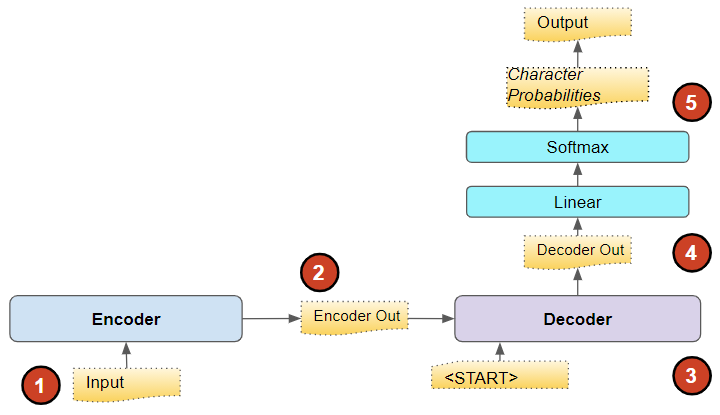
The model takes the source sentence as its input and passes it through an Embedding layer followed by an Encoder. The Encoder then outputs an encoded representation that compactly captures the essential features of the input.

This representation is then fed to a Decoder along with a “<START>” token to seed its output. The Decoder uses these to generate its own output, which is an encoded representation of the sentence in the target language.

This is then passed through an output layer, which might consist of some Linear layers followed by a Softmax. The Linear layers output a score of the likelihood of occurrence of each word in the vocabulary, at each position in the output sequence. The Softmax then converts those scores into probabilities.

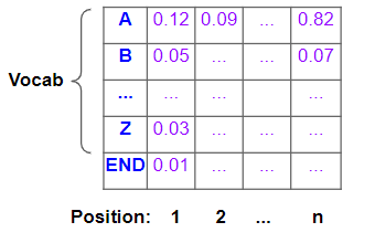
Probabilities for each character in the vocabulary, for each position in the output sequence (Image by Author)

Our eventual goal, of course, is not these probabilities but a final target sentence. To get that, the model has to decide which word it should predict for each position in that target sequence.

The model predicts an output sentence based on the probabilities (Image by Author)

How does it do that?

Greedy Search

A fairly obvious way is to simply take the word that has the highest probability at each position and predict that. It is quick to compute and easy to understand, and often does produce the correct result.

Greedy Search (Image by Author)

In fact, Greedy Search is so easy to understand, that we don’t need to spend more time explaining it 😃. But can we do better?

Aha, finally that brings us to our real topic!

Beam Search

Beam Search makes two improvements over Greedy Search.

• With Greedy Search, we took just the single best word at each position. In contrast, Beam Search expands this and takes the best ’N’ words.
• With Greedy Search, we considered each position in isolation. Once we had identified the best word for that position, we did not examine what came before it (ie. in the previous position), or after it. In contrast, Beam Search picks the ’N’ best sequences so far and considers the probabilities of the combination of all of the preceding words along with the word in the current position.

In other words, it is casting the “light beam of its search” a little more broadly than Greedy Search, and this is what gives it its name. The hyperparameter ’N’ is known as the Beam width.

Intuitively it makes sense that this gives us better results over Greedy Search. Because, what we are really interested in is the best complete sentence, and we might miss that if we picked only the best individual word in each position.

Beam Search — What it does

Let’s take a simple example with a Beam width of 2, and using characters to keep it simple.

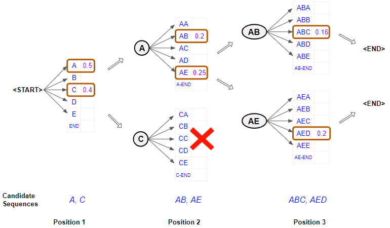
Beam Search example, with width = 2 (Image by Author)

First Position

• Consider the output of the model at the first position. It starts with the “<START>” token and obtains probabilities for each word. It now selects the two best characters in that position. eg. “A” and “C”.

Second Position

• When it comes to the second position, it re-runs the model twice to generate probabilities by fixing the possible characters in the first position. In other words, it constrains the characters in the first position to be either an “A” or a “C” and generates two branches with two sets of probabilities. The branch with the first set of probabilities corresponds to having “A” in position 1, and the branch with the second set corresponds to having “C” in position 1.
• It now picks the overall two best character pairs based on the combined probability of the first two characters, from out of both sets of probabilities. So it doesn’t pick just one best character pair from the first set and one best character pair from the second set. eg. “AB” and “AE”

Third Position

• When it comes to the third position, it repeats the process. It re-runs the model twice by constraining the first two positions to be either “AB” or “AE” and again generates two sets of probabilities.
• Once more, it picks the overall two best character triplets based on the combined probability of the first three characters from both sets of probabilities. Therefore we now have the two best combinations of characters for the first three positions. eg. “ABC” and “AED”.

Repeat till END token

• It continues doing this till it picks an “<END>” token as the best character for some position, which then concludes that branch of the sequence.

It finally ends up with the two best sequences and predicts the one with the higher overall probability.

Beam Search — How it works

We now understand Beam Search at a conceptual level. Let’s go one level deeper and understand the details of how this works. We’ll continue with the same example and use a Beam width of 2.

Continuing with our sequence-to-sequence model, the Encoder and Decoder would likely be a recurrent network consisting of some LSTM layers. Alternately it could also be built using Transformers rather than a recurrent network.

An LSTM-based Sequence-to-Sequence model (Image by Author)

Let’s focus on the Decoder component and the output layers.

First Position

In the first timestep, it uses the Encoder’s output and an input of a “<START>” token to generate the character probabilities for the first position.

Character probabilities for the first position (Image by Author)

Now it picks two characters with the highest probability eg. “A” and “C”.

Second Position

For the second timestep, it then runs the Decoder twice using the Encoder’s output as before. Along with the “<START>” token in the first position, it forces the input of the second position to be “A” in the first Decoder run. In the second Decoder run, it forces the input of the second position to be “C”.

Character probabilities for the second position (Image by Author)

It generates character probabilities for the second position. But these are individual character probabilities. It needs to compute the combined probabilities for character pairs in the first two positions. The probability of the pair “AB” is the probability of “A” occurring in the first position multiplied by the probability of “B” occurring in the second position, given that “A” is already fixed in the first position. The example below shows the calculation.

Calculate probabilities for character-pairs in the first two positions (Image by Author)

It does this for both Decoder runs and picks the character pairs with the highest combined probabilities across both runs. It, therefore, picks “AB” and “AE”.

The model picks the two best character pairs based on the combined probability (Image by Author)

Third Position

For the third time step, it again runs the Decoder twice as before. Along with the “<START>” token in the first position, it forces the input of the second position and third positions to be “A” and “B” respectively in the first Decoder run. In the second Decoder run, it forces the input of the second position and third positions to be “A” and “E” respectively.

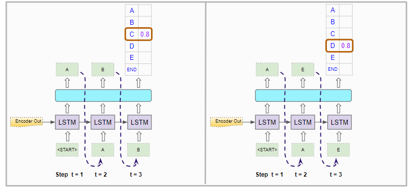
Character probabilities for the third position (Image by Author)

It calculates the combined probability for character triples in the first three positions.

Calculate probabilities for character-triples in the first three positions (Image by Author)

It picks the two best ones across both runs, and therefore picks “ABC” and “AED”.

The model picks the two best character triples based on the combined probability (Image by Author)

Repeat till END token

It repeats this process till it generates two best sequences that end with an “<END>” token.

It then chooses the sequence that has the highest combined probability to make its final prediction.

Conclusion

This gives us a sense of what Beam Search does, how it works, and why it gives us better results. This comes at the expense of increased computation, and longer execution times. So we should evaluate whether that tradeoff makes sense for our application’s use case.