xgboost参考

原文链接 https://zhuanlan.zhihu.com/p/51047761

二元分类实战——人口普查数据集的预测分类

和鲸社区Kesci

Connect People with Data.

8 人赞同了该文章

本篇notebook将介绍如何使用逻辑回归、朴素贝叶斯、以及XGBoost来构建二元分类器，预测居民收入是否超过50K$/year。特征选取、调参也会用来优化模型。

想要深入学习的小伙伴们可以点击原项目链接，一键Fork到自己的工作区，在线开展数据分析~

 

项目连接：人口普查数据集的预测分类
数据集：人口普查收入数据集（UCI）
作者：小科

 

• 在这篇notebook中，我们会将income_census_train.csv文件数据看做整个数据集，原因会在后续的内容中 阐述。
• 在进行特征工程等预处理后，我们会使用Logitic Regression、GussianNB来构建并训练模型；
• 同时，我们会使用未经过特征选取的数据作为XGBoost模型的训练的输入，并利用GridSearchCV进行调参。在找到我们所需要的最有参数后，应用XGBoost原生的形式训练，因为这样可以实现性能的提升，加上early stopping达到防止过拟合的效果。
• 生的形式训练，因为这样可以实现性能的提升，加上early stopping达到防止过拟合的效果。

数据探索

数据集实例数与特征数，缺失值查看等

• 原训练集shape: (30162, 16)
• 原测试集shape: (15060, 15)
• 原数据集实例数： 45222

缺失值检测

• 原训练集： 0
• 原测试集： 0

所有字段名

Index(['ID', 'age', 'workclass', 'fnlwgt', 'education', 'education_num', 'marital_status', 'occupation', 'relationship', 'race', 'gender', 'capital_gain', 'capital_loss', 'hours_per_week', 'native_country', 'income_bracket'], dtype='object')

# 各个特征的描述与相关总结
data_train.describe()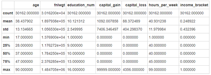

展示所有类型特征

data_train.describe(include=['O'])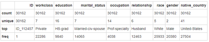

查看8个categorial数据类型的属性唯一值

workclass: 7 个
['State-gov' 'Self-emp-not-inc' 'Private' 'Federal-gov' 'Local-gov' 'Self-emp-inc' 'Without-pay']
education: 16 个 ['Bachelors' 'HS-grad' '11th' 'Masters' '9th' 'Some-college' 'Assoc-acdm' '7th-8th' 'Doctorate' 'Assoc-voc' 'Prof-school' '5th-6th' '10th' 'Preschool' '12th' '1st-4th']
marital_status: 7 个 ['Never-married' 'Married-civ-spouse' 'Divorced' 'Married-spouse-absent' 'Separated' 'Married-AF-spouse' 'Widowed']
occupation: 14 个 ['Adm-clerical' 'Exec-managerial' 'Handlers-cleaners' 'Prof-specialty' 'Other-service' 'Sales' 'Transport-moving' 'Farming-fishing' 'Machine-op-inspct' 'Tech-support' 'Craft-repair' 'Protective-serv' 'Armed-Forces' 'Priv-house-serv']
relationship: 6 个 ['Not-in-family' 'Husband' 'Wife' 'Own-child' 'Unmarried' 'Other-relative']
race: 5 个 ['White' 'Black' 'Asian-Pac-Islander' 'Amer-Indian-Eskimo' 'Other']
gender: 2 个 ['Male' 'Female']
native_country: 41 个 ['United-States' 'Cuba' 'Jamaica' 'India' 'Mexico' 'Puerto-Rico' 'Honduras' 'England' 'Canada' 'Germany' 'Iran' 'Philippines' 'Poland' 'Columbia' 'Cambodia' 'Thailand' 'Ecuador' 'Laos' 'Taiwan' 'Haiti' 'Portugal' 'Dominican-Republic' 'El-Salvador' 'France' 'Guatemala' 'Italy' 'China' 'South' 'Japan' 'Yugoslavia' 'Peru' 'Outlying-US(Guam-USVI-etc)' 'Scotland' 'Trinadad&Tobago' 'Greece' 'Nicaragua' 'Vietnam' 'Hong' 'Ireland' 'Hungary' 'Holand-Netherlands']

注意：在这里由于原数据集文件中的测试集文件是不包含label数据的，所以在这篇notebook中，我们会将原训练集看做整个数据集。

数据预处理

数字化类别数据

将有顺序的数据类型编码至分类数据（Ordinal Encoding to Categoricals）

• 比如，在education特征中，值HS-grad,Bachelors,Masters等是有顺序的。

# 将oject数据转化为int类型
for feature in data.columns:
    if data[feature].dtype == 'object':
        data[feature] = pd.Categorical(data[feature]).codes # codes	这个分类的分类代码

data.head()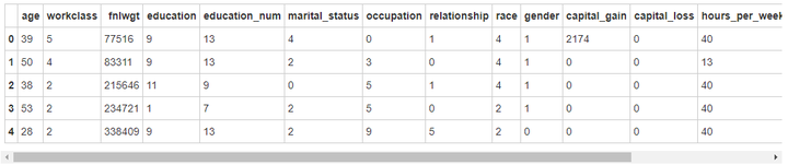

此时在查看数据每个字段的数值类型都是int类型。

data.info()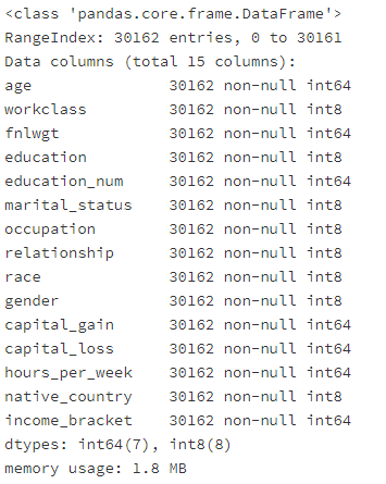

选取特征数据与类别数据

from sklearn.preprocessing import StandardScaler
from sklearn.linear_model import LogisticRegression
from sklearn.model_selection import train_test_split

X_df = data.iloc[:,data.columns != 'income_bracket']
y_df = data.iloc[:,data.columns == 'income_bracket']

X = np.array(X_df)
y = np.array(y_df)

标准化数据

scaler = StandardScaler()
X = scaler.fit_transform(X)

特征选取（Feature Selection）

特征重要性评估

在这里我们使用DecisionTreesClassifier来判断特征变量的重要性

from sklearn.tree import DecisionTreeClassifier
# from sklearn.decomposition import PCA

# fit an Extra Tree model to the data
tree = DecisionTreeClassifier(random_state=0)
tree.fit(X, y)

# 显示每个属性的相对重要性得分
relval = tree.feature_importances_

 

trace = Bar(x = X_df.columns.tolist(), y = relval, text = [round(i,2) for i in relval], textposition= "outside", marker = dict(color = colors))
iplot(Figure(data = [trace], layout = Layout(title="特征重要性", width = 800, height = 400, yaxis = dict(range = [0,0.25]))))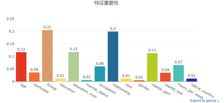

递归特征消除 (RFE)

选取10个重要特征

from sklearn.feature_selection import RFE

# 使用决策树作为模型
lr = DecisionTreeClassifier()
names = X_df.columns.tolist()

# 将所有特征排序
selector = RFE(lr, n_features_to_select = 10)
selector.fit(X,y.ravel())

print("排序后的特征：",sorted(zip(map(lambda x:round(x,4), selector.ranking_), names)))

排序后的特征： [(1, 'age'), (1, 'capital_gain'), (1, 'capital_loss'), (1, 'education_num'), (1, 'fnlwgt'), (1, 'hours_per_week'), (1, 'occupation'), (1, 'race'), (1, 'relationship'), (1, 'workclass'), (2, 'native_country'), (3, 'education'), (4, 'marital_status'), (5, 'gender')]

# 得到新的dataframe
X_df_new = X_df.iloc[:, selector.get_support(indices = False)]
X_df_new.columns

标准化特征选取后的数据 + 训练集与测试集切分

X_new = scaler.fit_transform(np.array(X_df_new)) # 数组化 + 标准化
X_train, X_test, y_train, y_test = train_test_split(X_new,y) # 切分

建模 + 评估

from sklearn.linear_model import LogisticRegression
from sklearn.naive_bayes import GaussianNB
from sklearn import metrics
from sklearn.metrics import confusion_matrix,roc_curve, auc, recall_score, classification_report

import matplotlib.pyplot as plt

 

import itertools

# 绘制混淆矩阵
def plot_confusion_matrix(cm, classes,
                          title='Confusion matrix',
                          cmap=plt.cm.Blues):
    """
    This function prints and plots the confusion matrix.
    Normalization can be applied by setting `normalize=True`.
    """
    plt.imshow(cm, interpolation='nearest', cmap=cmap)
    plt.title(title)
    plt.colorbar()
    tick_marks = np.arange(len(classes))
    plt.xticks(tick_marks, classes, rotation=0)
    plt.yticks(tick_marks, classes)

    thresh = cm.max() / 2.
    for i, j in itertools.product(range(cm.shape[0]), range(cm.shape[1])):
        plt.text(j, i, cm[i, j],
                 horizontalalignment="center",
                 color="white" if cm[i, j] > thresh else "black")

    plt.tight_layout()
    plt.ylabel('True label')
    plt.xlabel('Predicted label')

1. 逻辑回归（Logistic Regression）

# instance
lr = LogisticRegression()
# fit
lr_clf = lr.fit(X_train,y_train.ravel())
# predict
y_pred = lr_clf.predict(X_test)

print('LogisticRegression %s' % metrics.accuracy_score(y_test, y_pred))

LogisticRegression 0.8171330062325951

cm = confusion_matrix(y_test, y_pred)

class_names = [0,1]
plt.figure()
plot_confusion_matrix(cm , classes=class_names, title='Confusion matrix')
plt.show()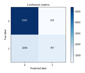

2. 先验为高斯分布的朴素贝叶斯（GussianNB）

gnb = GaussianNB()
gnb_clf = gnb.fit(X_train, y_train.ravel())
y_pred2 = gnb_clf.predict(X_test)

print('GaussianNB %s' % metrics.accuracy_score(y_test, y_pred2))

GaussianNB 0.7887548070547673

cm = confusion_matrix(y_test, y_pred2)

class_names = [0,1]
plt.figure()
plot_confusion_matrix(cm , classes=class_names, title='Confusion matrix')
plt.show()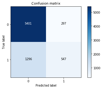

3. XGBoost

X_train, X_test, y_train, y_test = train_test_split(X_df_new,y) # 切分
X_train_std = scaler.fit_transform(X_train) # 标准化
X_test_std = scaler.fit_transform(X_test) # 标准化

调参

用GridSearchCV进行模型调参 [2]

• 第一次调参：'max_depth': [3, 5, 7], 'min_child_weight': [1, 3, 5]
• 结果： 最佳参数： {'max_depth': 7, 'min_child_weight': 3}
• 第二次调参：'learning_rate': [0.1,0.05, 0.01], 'subsample': [0.7,0.8,0.9]
• 最佳参数： {'learning_rate': 0.01, 'subsample': 0.8}

from xgboost import XGBClassifier
from sklearn.model_selection import GridSearchCV

 

cv_params = {'max_depth': [3, 5, 7], 'min_child_weight': [1, 3, 5]}
ind_params = {'learning_rate': 0.1, 'n_estimators': 1000, 'seed': 0,
              'subsample': 0.8, 'colsample_bytree': 0.8,
              'objective': 'binary:logistic'}

xgbm_gsearch1 = GridSearchCV(estimator=XGBClassifier(ind_params), 
                    param_grid=cv_params,
                    scoring='accuracy', cv=5, n_jobs=-1)
                         
xgb_optimized_clf = xgbm_gsearch1.fit(X_train_std, y_train.ravel())

 

# 最佳参数
print('最佳参数：',xgb_optimized_clf.best_params_)

for params, mean_score, scores in xgb_optimized_clf.grid_scores_:
    print("%0.3f (+/-%0.03f) for %r"
          % (mean_score, scores.std() * 2, params))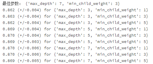

# 预测测试集数据
y_pred3 = xgb_optimized_clf.predict(X_test_std)

print(classification_report(y_test,y_pred3))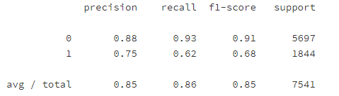

根据上面调参后的结果，得到最佳参数为'max_depth'=7, 'min_child_weight'=3, 接下来固定模型的这两个参数，调整参数'learning rate'与'subsample'的值。继续优化模型。

cv_params_new = {'learning_rate': [0.1,0.05, 0.01], 'subsample': [0.7,0.8,0.9]}

 

xgbm_gsearch2 = GridSearchCV(
                        estimator=XGBClassifier(
                                    max_depth=7, min_child_weight=1,
                                    n_estimators=1000, seed=0, colsample_bytree=0.8,
                                    objective='binary:logistic'
                                    ),
                         param_grid=cv_params_new,
                         scoring='accuracy', cv=5, n_jobs=-1)
                         
xgb_optimized_clf = xgbm_gsearch2.fit(X_train_std, y_train.ravel())

 

# 最佳参数
print('最佳参数：',xgb_optimized_clf.best_params_)

for params, mean_score, scores in xgb_optimized_clf.grid_scores_:
    print("%0.3f (+/-%0.03f) for %r" % (mean_score, scores.std() * 2, params))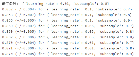

# 预测
y_pred4 = xgb_optimized_clf.predict(X_test_std)
print('XGBoost Accuracy %s' % metrics.accuracy_score(y_test, y_pred4))
print(classification_report(y_test, y_pred4))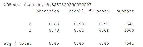

XGBoost Early Stopping CV

直接使用上面 调参得出的4个最佳参数，并用Early Stopping CV来防止xgboost模型过拟合。

import xgboost as xgb

# X_train, y_train： dataframe
# 加载dataframe数据，并存储到DMatrix中，也可以加载csv、libsvm文件，使得XGBoost更高效
xgb_matrix = xgb.DMatrix(X_train, y_train) 
params = {'max_depth': 7, 'min_child_weight': 3, 
            'subsample': 0.8, 'learning_rate': 0.01,
            'n_estimators':1000, 'seed':0, 
            'colsample_bytree':0.8,'objective':'binary:logistic'
}
cv_xgb = xgb.cv(params = params, dtrain=xgb_matrix, num_boost_round=3000, nfold=5, metrics=['error'],
                early_stopping_rounds=100) # early stooping来最小化error
# 查看输出结果最后五行：
print(cv_xgb.tail(5))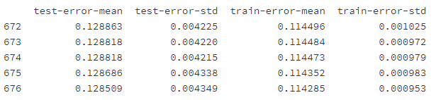

训练后的特征重要性
根据上面 5行的显示结果，最后设定num_boost_round为 676 来训练我们最终的xgboost模型,并绘制特征重要性排名

final_xgb_model = xgb.train(params=params, dtrain=xgb.DMatrix(X_train, y_train), num_boost_round=676)
%matplotlib inline
import seaborn as sns
sns.set(font_scale = 1.5)

xgb.plot_importance(final_xgb_model)
plt.show()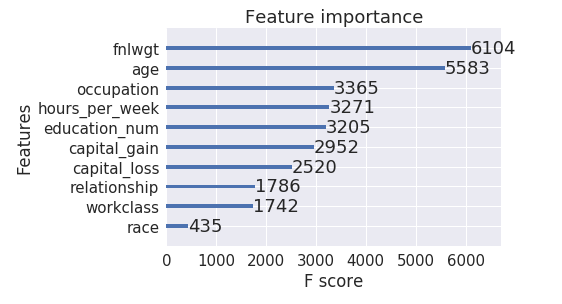 

现在我们也可以根据得到的特征重要性字典绘制我们自己的图。

feature_importance_dict = final_xgb_model.get_fscore()
feature_importance_dict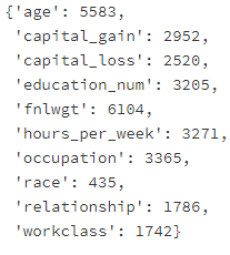

feature_importance_df = pd.DataFrame({'Importance':list(feature_importance_dict.values()),
                                        'Feature':list(feature_importance_dict.keys()),
                                    })
feature_importance_df.sort_values(by = ['Importance'], inplace=True)
feature_importance_df.plot(kind = 'barh', x = 'Feature', figsize = (8,8), color = 'orange')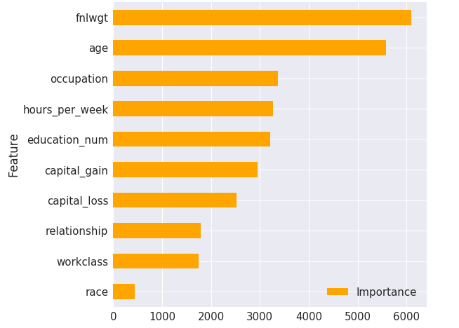

分析在测试集上的性能

# 预测
test_mat = xgb.DMatrix(X_test)
y_pred5 = final_xgb_model.predict(test_mat)
y_pred5

将概率转变为类别

y_pred5[y_pred5>0.5] = 1
y_pred5[y_pred5<=0.5] = 0
y_pred5

模型评估

• 准确率

print('XGBoost Accuracy {0:.2%}'.format(metrics.accuracy_score(y_test, y_pred5)))

• 分类报告

print(classification_report(y_test, y_pred4))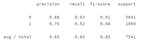

• 混淆矩阵

cm = confusion_matrix(y_test, y_pred5)

class_names = [0,1]
plt.figure()
plot_confusion_matrix(cm , classes=class_names, title='Confusion matrix')
plt.show()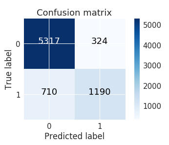

参考

• https://www.kaggle.com/marksman/us-adult-income-salary-prediction
• https://blog.csdn.net/haluoluo211/article/details/78943332
• Gradient Boosted Trees with XGBoost
• https://www.kaggle.com/chekoduadarsh/hybrid-cnn-xgboost-gnb-accuracy-99
• https://segmentfault.com/a/1190000014040317