【共振峰跟踪】通过平均不同分辨率的方法跟踪共振峰，基于时频lpc的频谱图的MATLAB仿真

1.软件版本

MATLAB2021a

 

2.本算法理论知识

通过平均不同分辨率的方法跟踪共振峰，基于时频lpc的频谱图。此外，它还决定了语音信号的基音轮廓。

3.核心代码

function [fmap,pt2] = ftrack(y,fs)


bDisplay = 1;

Fsamps = 256; % sampling resolution in frequency dimension
Tsamps = round(length(y)/18000*256); % sampling resolution in time dimension


tmp_img1 = zeros(Fsamps,Tsamps);
ct = 0;

numiter = 8; % number of iterations to run. seemed like a good number



for i=2.^(8-8*exp(-linspace(1.5,10,numiter)/1.4)),
% Determine the time-frequency distribution at the current

fix(length(y)/round(i))
round(i)
[tmp_img1,ft1,pt1] = lpcsgram(y,fix(length(y)/round(i)),round(i),fs);

% Get the dimensions of the output time-frequency image
[M,N] = size(tmp_img1);

% Create a grid of the final resolution
[xi,yi] = meshgrid(linspace(1,N,Tsamps),linspace(1,M,Fsamps));

% Interpolate returned TF image to final resolution
tmp_img2 = interp2(tmp_img1,xi,yi);

ct = ct+1;

% Interpolate formant tracks and pitch tracks
pt2(:,ct) = interp1([1:length(pt1)]',pt1(:),linspace(1,length(pt1),Tsamps)');
ft2(:,:,ct) = interp1(linspace(1,length(y),fix(length(y)/round(i)))',Fsamps*ft1',linspace(1,length(y),Tsamps)')';

% Normalize
tmp_img3(:,:,ct) = tmp_img2/max(tmp_img2(:));

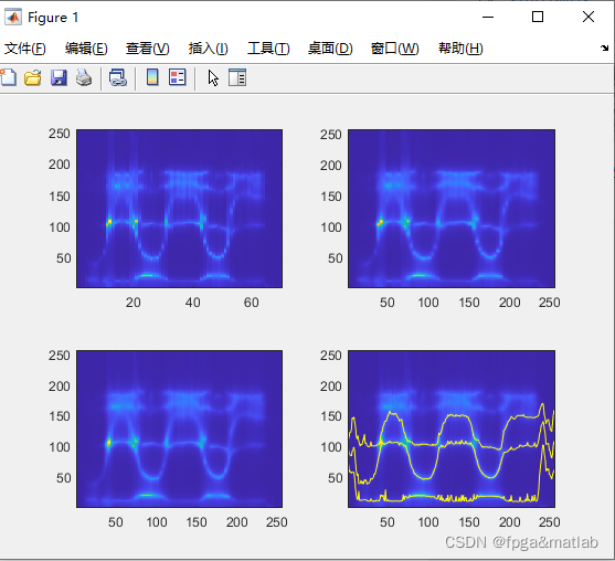
if bDisplay,
subplot(221);imagesc(tmp_img1);axis xy;
subplot(222);imagesc(tmp_img2);axis xy;
subplot(223);imagesc(squeeze(mean(tmp_img3,3)));axis xy;
drawnow;
end;
end

% Determine mean tfr image and formant track
tmp_img4 = squeeze(mean(tmp_img3,3)); % tfr
ft3 = squeeze(nanmean(permute(ft2,[3 2 1]))); %

if bDisplay,
subplot(224);imagesc(tmp_img4);axis xy;
hold on;
plot(ft3,'y');
end;

% convert fmnts to image
tmap = repmat([1:Tsamps]',1,3);
idx = find(~isnan(sum(ft3,2)));
fmap = ft3(idx,:);
tmap = tmap(idx,:);
% filter formant tracks to remove noise
[b,a] = butter(9,0.1);
fmap = round(filtfilt(b,a,fmap));
pt3 = nanmean(pt2');
pt3 = (pt3-nanmin(pt3))/(nanmax(pt3)-nanmin(pt3));

% Rescaling is done after display code
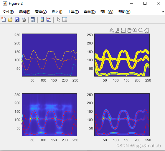
if bDisplay,
imap = zeros(Fsamps,Tsamps);
ind = sub2ind(size(imap),fmap(:),tmap(:));
imap(ind) = 1;

tpts = tmap(:,1);

figure;
subplot(221);
imagesc(imap);axis xy;hold on;
plot(tpts,fmap(:,1),tpts,fmap(:,2),tpts,fmap(:,3));
idx = [1:5]';
plot(tpts(idx),fmap(idx,1),'.-',tpts(idx),fmap(idx,2),'.-',tpts(idx),fmap(idx,3),'.-');

subplot(222);

% Create a wider formant track
anisomask = anisodiff(imap,6,50,0.01,1);

imagesc(anisomask>0);axis xy;hold on;
plot(tpts,fmap(:,1),tpts,fmap(:,2),tpts,fmap(:,3));
idx = [1:5]';
plot(tpts(idx),fmap(idx,1),'.-',tpts(idx),fmap(idx,2),'.-',tpts(idx),fmap(idx,3),'.-');

subplot(223);
imagesc(tmp_img4);axis xy;hold on;
plot(tpts,fmap(:,1),'r',tpts,fmap(:,2),'r',tpts,fmap(:,3),'r');
idx = [1:5]';
plot(tpts(idx),fmap(idx,1),'.-',tpts(idx),fmap(idx,2),'.-',tpts(idx),fmap(idx,3),'.-');

subplot(224);
imagesc(tmp_img4.*(anisomask>0));axis xy;hold on;
plot(tpts,fmap(:,1),'r-',tpts,fmap(:,2),'r-',tpts,fmap(:,3),'r-');
% idx = [1:5]';
% plot(tpts(idx),fmap(idx,1),'.-',tpts(idx),fmap(idx,2),'.-',tpts(idx),fmap(idx,3),'.-');
plot(256*pt3,'y.-');
end;

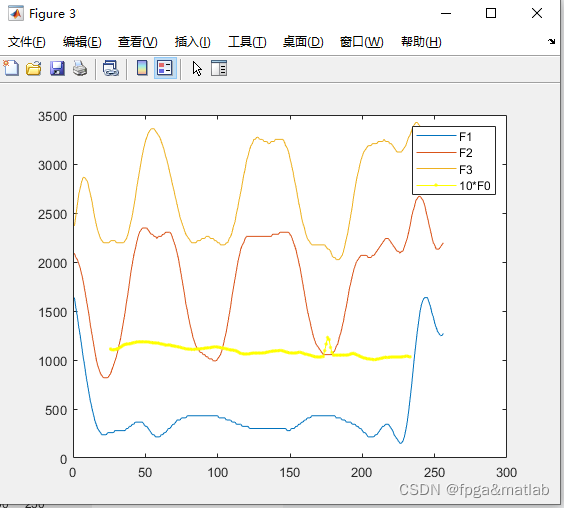
% Rescale to Actual Formants and take the mean of pitch tracks
fmap = (fs/2)*(fmap/256);
pt2 = nanmean(pt2');

4.操作步骤与仿真结论

 

 

 

 

 

 D201