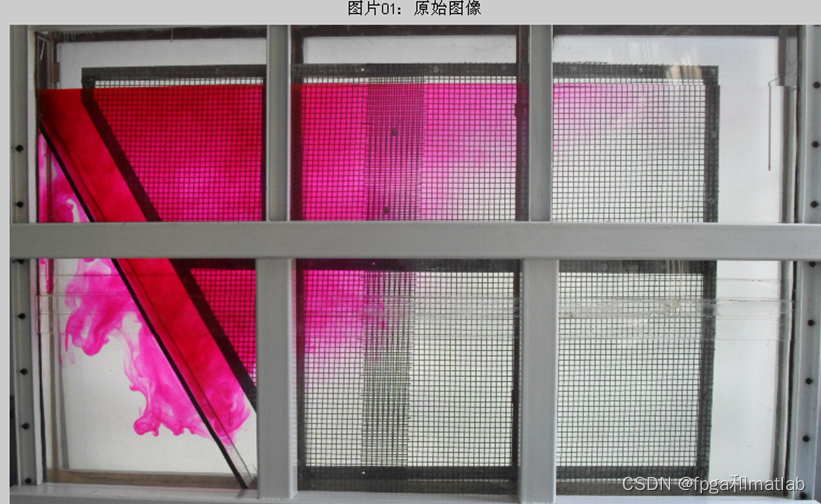
使用matlab根据液体扩散图片分析其对应的等浓度线
目录
一、理论基础
二、核心程序
三、仿真测试结果
作者ID :fpga和matlab
CSDN主页:https://blog.csdn.net/ccsss22?type=blog
擅长技术:
1.无线基带,无线图传,编解码
2.机器视觉,图像处理,三维重建
3.人工智能,深度学习
4.智能控制,智能优化
5.其他
一、理论基础
第一步:图像预处理。滤波,光照不均匀处理等等。
一般对于光泽处理我们采用同态滤波的方法来实现,这里图像预处理主要就是光照不均匀的处理。现实中我们得到的图片,其动态范围很大,而我们感兴趣的部分的灰度又很暗,图像细节没有办法辨认,采用一般的灰度级线性变换法是不行的。图像的同态滤波属于图像频率域处理范畴,其作用是对图像灰度范围进行调整,通过消除图像上照明不均的问题,增强暗区的图像细节,同时又不损失亮区的图像细节.分辨不清的图像用同态滤波器处理后,图像画面亮度比较均匀,细节得以增强。
第二步:去本底。提取红色液体,排除背景的影响。建议:从色度方面考虑,色度的原理大致要说明。
这里我们采用HSV提取色度。其代码更为简单。
phsv = rgb2hsv(I1);
ph = phsv(:,:,1); % 取H分量
ps = phsv(:,:,2); % 取S分量
pv = phsv(:,:,3); % 取V分量
%=====================================================================
figure;
subplot(221);subimage(I1); colorbar; %显示原rgb图像
Xlabel('(a) rgb图像','FontSize',14,'FontName','隶书','color','b');
subplot(222);subimage(ph); colorbar; %显示色调分量图像
Xlabel('(b) 色调分量图像','FontSize',14,'FontName','隶书','color','b');
subplot(223);subimage(ps); colorbar; %显示饱和度分量图像
Xlabel('(c) 饱和度分量图像','FontSize',14,'FontName','隶书','color','b');
subplot(224);subimage(pv); colorbar; %显示亮度分量图像
Xlabel('(d) 亮度分量图像','FontSize',14,'FontName','隶书','color','b');
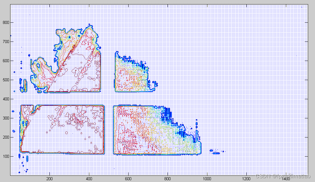
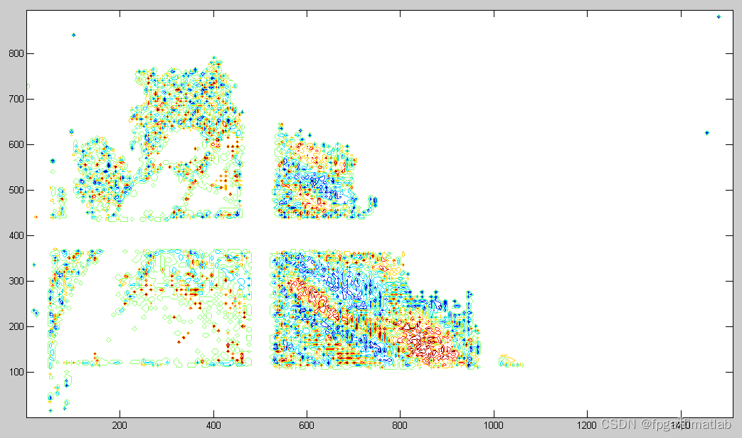
第三步:等浓度线图,填充颜色,根据等浓度线得出我给的EZ,EY值,用相同情况下的图片验证EZ,EY值的正确性。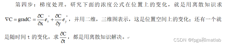
二、核心程序
。。。。。。。。。。。。。。。。。。。。。。。。。。。。。。。。。。
[R,C,K]= size(I);
if R == 1080
R2 = 900;
end
if R < 1080
R2 = R;
end
step = 5;%大的图片设置为5;
%第一步
%第一步
%第一步:图像预处理。滤波,光照不均匀处理等等。(用均值和中值滤波之外的方法,
% 至少两种滤波方法和两种光照不均匀处理的方法)。
%采用同态滤波
I1=tongtai(I,1,0.4,R2,C);
% pause(2)%暂停3秒钟后关闭第一步的处理图片;
% close all;
% % 顺序统计滤波
% Ri=I(:,:,1);
% Gi=I(:,:,2);
% Bi=I(:,:,3);
%
% Rpstatistic=mystatistic(Ri);
% Gpstatistic=mystatistic(Gi);
% Bpstatistic=mystatistic(Bi);
%
% I1(:,:,1)=Rpstatistic(:,:);
% I1(:,:,2)=Gpstatistic(:,:);
% I1(:,:,3)=Bpstatistic(:,:);
% imshow(I1)
%第二步
%第二步
%第二步:去本底。提取红色液体,排除背景的影响。
%通过对比,可以看到G图像对应的液体的视觉效果比较明显,所以我们通过对G图像进行处理得到液体的范围;
%这里有两种方法供使用,我们采用的是HSV法。
%这里有两种方法供使用,我们采用的是HSV法。
%这里有两种方法供使用,我们采用的是HSV法。
%第一种方法,采用的是腐蚀的方法提起图片;
% % % I2=im2double(I1);%将A转换成double型
% % % R=I2(:,:,1);
% % % G=I2(:,:,2);
% % % B=I2(:,:,3);
% % % fuzhuo(I1,G);
%==========================================================================
%第二种方法是采用HSV提取液体所在的图片
phsv = rgb2hsv(I1);
ph = phsv(:,:,1); % 取H分量
ps = phsv(:,:,2); % 取S分量
pv = phsv(:,:,3); % 取V分量
%==========================================================================
figure;
subplot(221);subimage(I1); colorbar; %显示原rgb图像
Xlabel('(a) rgb图像','FontSize',14,'FontName','隶书','color','b');
subplot(222);subimage(ph); colorbar; %显示色调分量图像
Xlabel('(b) 色调分量图像','FontSize',14,'FontName','隶书','color','b');
subplot(223);subimage(ps); colorbar; %显示饱和度分量图像
Xlabel('(c) 饱和度分量图像','FontSize',14,'FontName','隶书','color','b');
subplot(224);subimage(pv); colorbar; %显示亮度分量图像
Xlabel('(d) 亮度分量图像','FontSize',14,'FontName','隶书','color','b');
%液体的提取
%途中白色部分为液体的浓度变化
for i = 1:R2
for j = 1:C
if ps(i,j)<0.4
ps_tmp(i,j) = 0;
end
if ps(i,j)>0.4
ps_tmp(i,j) = ps(i,j);
end
end
end
figure
imshow(ps_tmp)
for i = 1:R2
for j = 1:C
ps_tmp2(i,j) = ps_tmp(i,j);
end
end
figure
imshow(ps_tmp2)
p1 = fushi2(ps_tmp2);%液体的浓度变换灰度图的腐蚀处理
% pause(2)%暂停3秒钟后关闭第一步的处理图片;
% close all;
% 第三步:等浓度线
% 第三步:等浓度线
% 第三步:等浓度线
for i = 1:R2
for j = 1:C
if p1(i,j)>0
if p1(i,j)<=0.2
nongdu(i,j,1) = 0;
nongdu(i,j,2) = 0;
nongdu(i,j,3) = 0;
end
end
if p1(i,j)>0.2
if p1(i,j)<=0.4
nongdu(i,j,1) = 255;
nongdu(i,j,2) = 255;
nongdu(i,j,3) = 0;
end
end
if p1(i,j)>0.4
if p1(i,j)<=0.6
nongdu(i,j,1) = 255;
nongdu(i,j,2) = 0;
nongdu(i,j,3) = 0;
end
end
if p1(i,j)>0.6
if p1(i,j)<=0.8
nongdu(i,j,1) = 0;
nongdu(i,j,2) = 0;
nongdu(i,j,3) = 255;
end
end
if p1(i,j)>0.8
if p1(i,j)<=1
nongdu(i,j,1) = 0;
nongdu(i,j,2) = 255;
nongdu(i,j,3) = 0;
end
end
if p1(i,j)==0
nongdu(i,j,1) = 0;
nongdu(i,j,2) = 0;
nongdu(i,j,3) = 0;
end
end
end
figure;
imshow(nongdu);
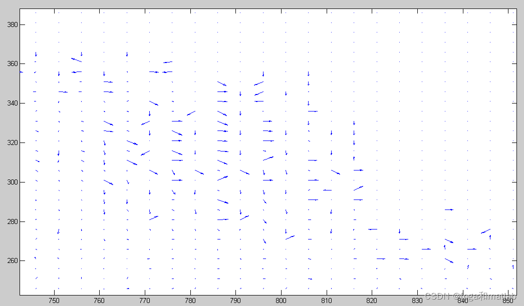
%第四步:梯度处理。
%第四步:梯度处理。
%第四步:梯度处理。
[Gx,Gy]=gradient(ps_tmp2); % 计算梯度
figure,imshow(Gx);
figure,imshow(Gy);
% G=sqrt(Gx.*Gx+Gy.*Gy); % 注意是矩阵点乘
% J1=G;
% figure,imshow(J1,map); % 第一种图像增强
%为了节约计算速率,这里每5个点计算一次
u = 1:step:R2;
v = 1:step:C;
for i=1:R2
for j=1:C
Gx2(i,j)=Gx(R2+1-i,j);
Gy2(i,j)=Gy(R2+1-i,j);
end
end
for i=1:R2
for j=1:C
ps_tmp22(i,j)=ps_tmp2(R2+1-i,j);
end
end
figure;quiver ( v,u,Gx2(1:step:R2,1:step:C),Gy2(1:step:R2,1:step:C) );
figure;contour( v,u,ps_tmp22(1:step:R2,1:step:C) );
u = 1:step:R2;
v = 1:step:C;
figure;contour( v,u,ps_tmp22(1:step:R2,1:step:C) );hold on;
quiver ( v,u,Gx2(1:step:R2,1:step:C),Gy2(1:step:R2,1:step:C) );
% pause(3)%暂停3秒钟后关闭第一步的处理图片;
% close all;
%第五步:旋度图。
[u v] = meshgrid(1:step:C,1:step:R2);
cav = curl(ps_tmp2(1:step:R2,1:step:C),v);
for i=1:R2/step
for j=1:C/step
cav2(i,j)=cav(R2/step-i+1,j);
end
end
figure;contour(v,u,cav2);
pcolor(u,v,cav2); shading interp;
colormap copper;
% hold on;
% quiver(ps_tmp2,ps_tmp2,u,v,'y');
%第六步:散度图。
figure
k=curvature_central(ps_tmp2);
imshow(k);
u = 1:step:R2;
v = 1:step:C;
for i=1:R2
for j=1:C
k2(i,j)=k(R2+1-i,j);
end
end
% figure;quiver ( v,u,Gx(1:5:900,2:5:1515),Gy(1:5:900,2:5:1515) );
figure;contour( v,u,k2(1:step:R2,1:step:C) );
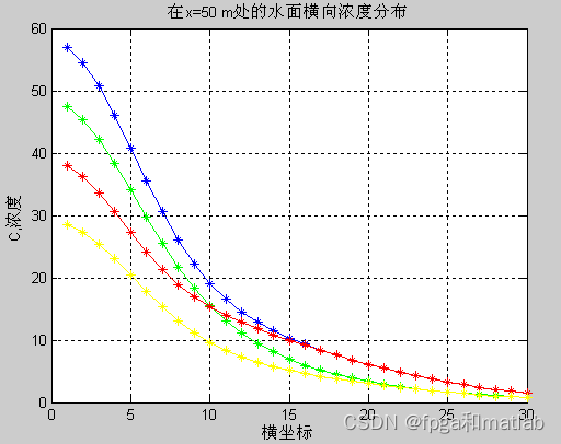
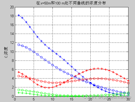
三、仿真测试结果
A16-02

 浙公网安备 33010602011771号