作业五——线性回归算法
【1.总结】
线性回归可以理解为:在N维空间中找一个形式像直线方程(y=ax+b)一样的函数来拟合数据。
因此,线性回归包括:
单元(单因素)线性回归
多元(多因素)线性回归
而在构建线性回归模型的过程中,我们需要选择最合适的那条线,即预测结果与真实结果误差最小,这里就涉及到一个概念:损失函数(最小二乘法)。
损失函数是模型输出和观测结果间概率分布差异的量化

其实质为欧式距离加和。
李航-《统计学习方法》中总结了“算法-策略-优化”模型,以下归纳线性回归算法的思想。

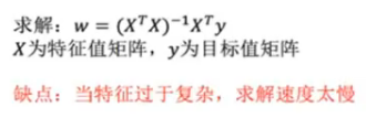
(1)所谓正规方程,
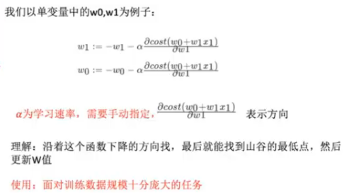
(2)所谓梯度下降,是对自变量进行不断的更新(针对w和b求偏导),使得目标函数不断逼近最小值的过程
【2.思考线性回归算法可以用来做什么?】
线性回归算法主要是学习已有数据集,预测后续发展。如可以根据气候条件等因素预测某地区日出时间。
【3.自主编写线性回归算法 ,数据可以自己造,或者从网上获取。(加分题)】
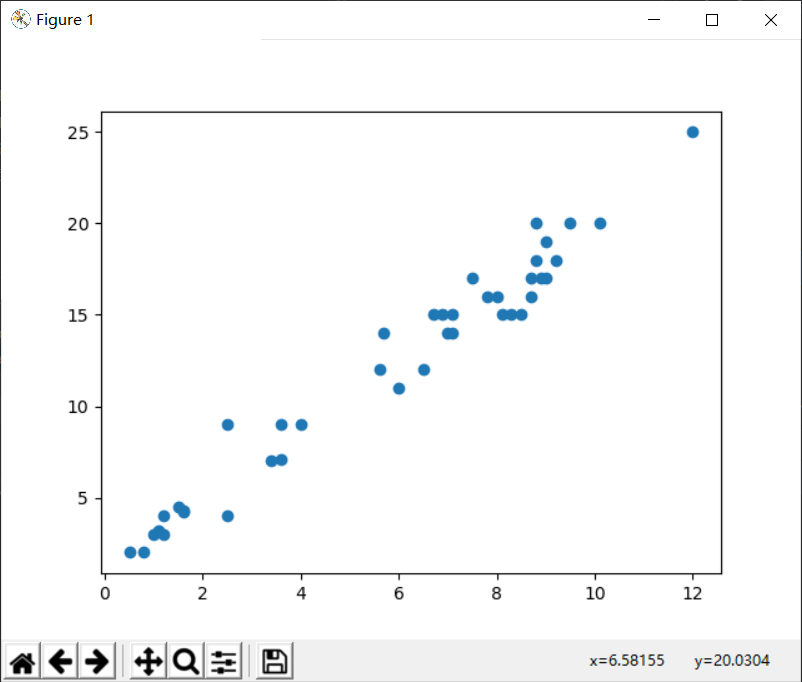
1)获取数据
 1 import pandas as pd
 2 import matplotlib.pyplot as plt
 3
 4
 5 points = pd.read_csv("E:/机器学习/机器学习及其算法/data/data.csv")
 6 # points
 7 # 提取points中的两列数据,分别作为x,y
 8 x = points.iloc[:, 0]
 9 y = points.iloc[:, 1]
10 x = x.values.reshape(1, -1)
11 y = y.values.reshape(1, -1)
12
13
14 # 用plt画出散点图
15 plt.scatter(x, y)
16 plt.show()
2)构造函数
· 损失函数
# 损失函数是系数的函数,另外还要传入数据的x,y
def compute_cost(w, b, points):
    total_cost = 0
    m = float(len(points))
    for i in range(len(points)):
        x = points.iloc[i, 0]
        y = points.iloc[i, 1]
        total_cost += (y - w * x - b) ** 2
    return total_cost / m  # 一除都是浮点
· 优化器——梯度下降
 1 def grad_desc(points, initial_w, initial_b, alpha, num_iter):
 2     # alpha为学习率,num_iter为迭代次数
 3     w = initial_w
 4     b = initial_b
 5     # 定义一个list保存所有的损失函数值,用来显示下降过程。
 6     cost_list = []
 7     for i in range(num_iter):
 8         cost_list.append(compute_cost(w, b, points))
 9         w, b = step_grad_desc(w, b, alpha, points)
10     return [w, b, cost_list]
· 参数更新——计算梯度
 1 def step_grad_desc(current_w, current_b, alpha, points):
 2     sum_grad_w = 0
 3     sum_grad_b = 0
 4     m = float(len(points))
 5     # 对每个点代入公式求和
 6     for i in range(len(points)):
 7         x = points.iloc[i, 0]
 8         y = points.iloc[i, 1]
 9         sum_grad_w += (current_w * x + current_b - y) * x
10         sum_grad_b += current_w * x + current_b - y
11     # 用公式求当前梯度
12     grad_w = 2 / m * sum_grad_w
13     grad_b = 2 / m * sum_grad_b
14
15     # 梯度下降,更新当前的w和b
16     updated_w = current_w - alpha * grad_w
17     updated_b = current_b - alpha * grad_b
18     return updated_w, updated_b
· 初始化数据
1 alpha = 0.0000001
2 initial_w = 0
3 initial_b = 0
4 num_iter = 20
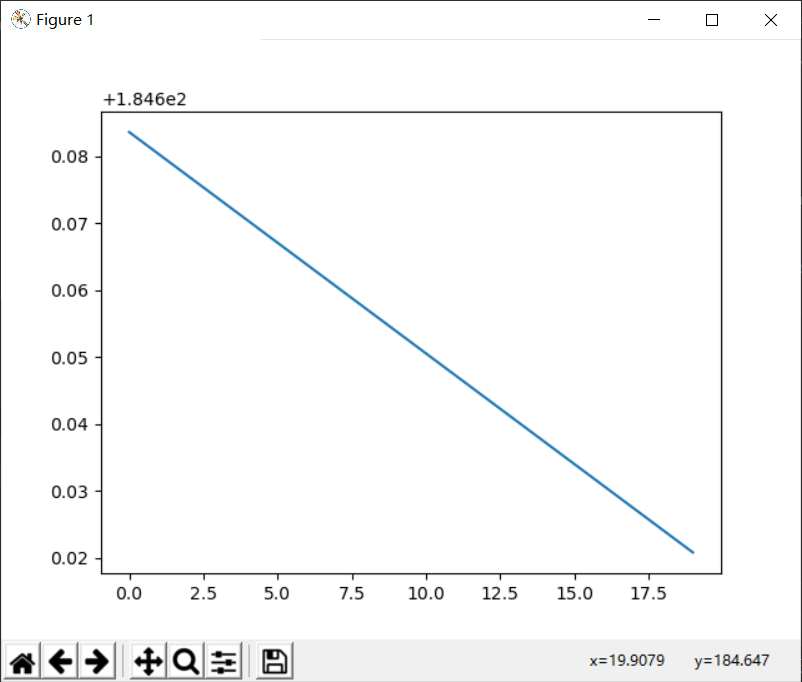
· 调用函数——计算w、b和损失值
 1 w, b, cost_list = grad_desc(points, initial_w, initial_b, alpha, num_iter)
 2 print("w is :", w)
 3 print("b is :", b)
 4
 5 cost = compute_cost(w, b, points)
 6
 7 print("cost_list:", cost_list)
 8 print("cost is:", cost)
 9 pred_y = w * x + b
10 plt.plot(cost_list)

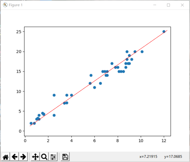
· 可视化——预测值与原始值
1 plt.scatter(x, y)
2 plt.plot(x, pred_y, c='r')
3 plt.show()
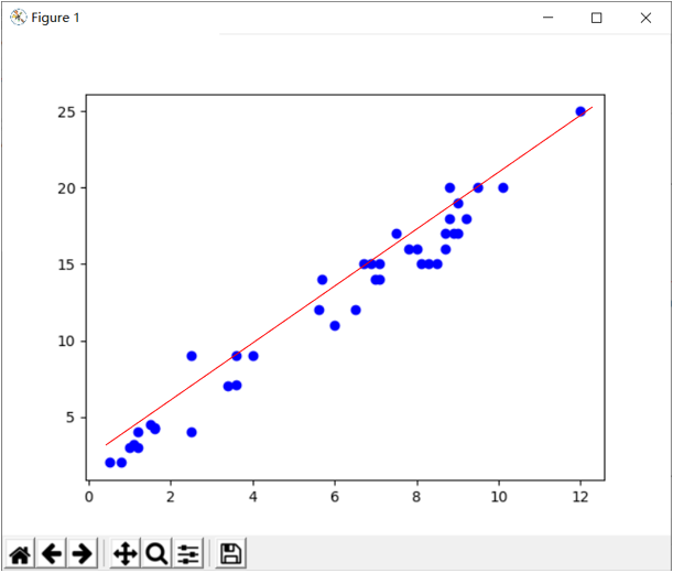
3)对比sklearn.LinearRegression
1 from sklearn.linear_model import LinearRegression
2
3 model = LinearRegression()
4 model.fit(x, y)
5 pre = model.predict(x)
6 plt.scatter(x, y, c='b')
7 plt.plot(x, pre, c='r')
8 plt.show()

 浙公网安备 33010602011771号