python 画直方图

# -*- coding: utf-8 -*-
import matplotlib.pyplot as plt
from datetime import datetime
import open_file

fig = plt.figure(figsize=(20, 10))

#  定义 x 轴数据
lat_x = [i for i in range(9, 55)]    
lon_x = [i for i in range(74, 135, 2)]
# 从文件读取数据
xn_lat, xn_lon = open_file.open_xn('int')
ys_lat, ys_lon = open_file.open_ys('int')
# 定义 y 轴数据
xn_lat_y = [i for i in map(lambda x: xn_lat.count(x)+ys_lat.count(x), lat_x)]   # 找到 lat_x 在数据 纬度xn_lat  中的个数  
xn_lon_y = [i for i in map(lambda x: xn_lon.count(x)+ys_lon.count(x), lon_x)]

ys_lat_y = [i for i in map(lambda x: ys_lat.count(x), lat_x)]
ys_lon_y = [i for i in map(lambda x: ys_lon.count(x), lon_x)]

dpi, width = 400, 0.4  # 分辨率，柱子宽度
plt.rc('font', family='SimHei', size=12)  # 设置中文显示,否则出现乱码
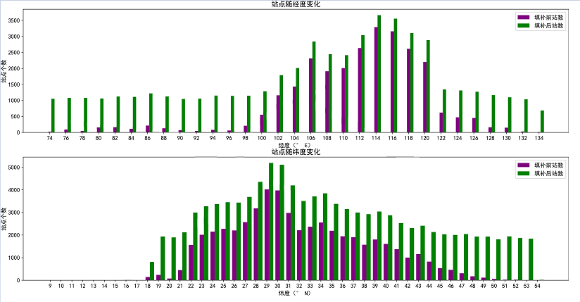
ax1 = plt.subplot(2, 1, 1)  # ('行','列','编号')  2 行 1 列 第 1 个 pu/rple
plt.bar(x=lon_x, height=ys_lon_y, width=width, label='填补前站数', fc='purple')
for i in range(len(lon_x)):   # 双柱图width  # 不加这段，双柱图会重叠，x 参数 其实就是设置它显示柱子的x轴的起始点，第一个为lon_x的 74 开始到加 width的0.4 结束  
    lon_x[i] = lon_x[i] + width                                                                    第二个为lon_x的 74+0.4 开始到加 width的0.4 结束

plt.bar(x=lon_x, height=xn_lon_y, width=width , label='填补后站数', fc='green')
plt.xticks([i for i in range(74, 135, 2)])  # 设置x轴上显示的值
# 设置横轴标签
plt.xlabel('经度（° E）')
# 设置纵轴标签
plt.ylabel('站点个数')
# 添加标题
plt.title('站点随经度变化')
plt.legend()  # 设置图例，就是让 label  画出来


ax2 = plt.subplot(2, 1, 2)  # ('行','列','编号')
plt.bar(x=lat_x, height=ys_lat_y, width=width, label='填补前站数', fc='purple')
for i in range(len(lat_x)):
    lat_x[i] = lat_x[i] + width
plt.bar(x=lat_x, height=xn_lat_y, width=width, label='填补后站数', fc='green')
plt.xticks([i for i in range(9, 55)])  # 设置x轴上显示的值

# 设置横轴标签
plt.xlabel('纬度（° N）')
# 设置纵轴标签
plt.ylabel('站点个数')
# 添加标题
plt.title('站点随纬度变化')
plt.legend()   # 让 label  画出来  loc='upper right'  设置图例在哪里



out_file = '%s_%s_%s.png' % (datetime.now().strftime('%Y%m%d%H%M&S'), width, dpi)
plt.savefig(out_file, transparent=True, bbox_inches='tight', dpi=dpi, pad_inches=0.0, set_visiable=False, format='png')
# plt.show()

 

import matplotlib.pyplot as plt
import numpy as np
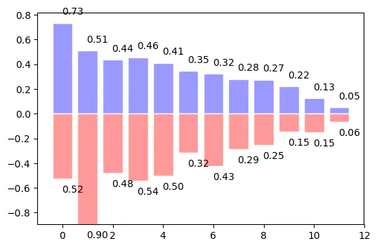
#柱状图分成上下两部分，每一个柱体上都有相应的数值标注，并且取消坐标轴的显示。
#向上向下分别生成12个数据，X为 0 到 11 的整数 ，Y是相应的均匀分布的随机数据。 
#使用的函数是plt.bar，参数为X和Y：
n = 12
X = np.arange(n)
Y1 = (1 - X / float(n)) * np.random.uniform(0.5, 1.0, n)
Y2 = (1 - X / float(n)) * np.random.uniform(0.5, 1.0, n)

plt.bar(X, +Y1)
plt.bar(X, -Y2)

plt.xlim(-.5, n)
plt.xticks(())
plt.ylim(-1.25, 1.25)
plt.yticks(())

plt.show()

#下面我们就颜色和数值进行优化。 用facecolor设置主体颜色，edgecolor设置边框颜色为白色
plt.bar(X, +Y1, facecolor='#9999ff', edgecolor='white')
plt.bar(X, -Y2, facecolor='#ff9999', edgecolor='white')
#接下来我们用函数plt.text分别在柱体上方（下方）加上数值，用%.2f保留两位小数，
#横向居中对齐ha='center'，纵向底部（顶部）对齐va='bottom'
for x, y in zip(X, Y1):
    # ha: horizontal alignment
    # va: vertical alignment
    plt.text(x + 0.4, y + 0.05, '%.2f' % y, ha='center', va='bottom')

for x, y in zip(X, Y2):
    # ha: horizontal alignment
    # va: vertical alignment
    plt.text(x + 0.4, -y - 0.05, '%.2f' % y, ha='center', va='top')

 

 

 

参数	说明	类型
x	x坐标	int,float
height	条形的高度	int,float
width	线条的宽度	0~1，默认是0.8
botton	条形的起始位置	也就是y轴的起始坐标
align	条形的中心位置	“center”,"lege"边缘
color	条形的颜色	“r”,“b”,“g”,“#123465",默认的颜色是“b”
edgecolor	边框的颜色	同上
linewidth	边框的宽度	像素，默认无，int
tick_label	下标的标签	可以是元组类型的字符组合
log	y轴使用科学计算法表示	bool
orientation	是竖直条还是水平条	竖直："vertical"，水平条："horizontal"

 

参考：https://www.jb51.net/article/142486.htm

           https://www.jianshu.com/p/364e2121ee94