二.机器学习算法篇-线性回归(1)
1.线性回归算法思想
机器学习算法可以分为有监督学习和无监督学习。
什么是有监督学习算法?
用已知某种或某些特性的样本作为训练集,以建立一个数学模型,再用已建立的模型来预测未知样本,此种方法被称为有监督学习,是最常用的一种机器学习方法。是从标签化训练数据集中推断出模型的机器学习任务。
回归算法是有监督学习算法的一种,从机器学习的角度来讲,回归算法用于构建一个算法模型,这个模型是属性(X)与标签(Y)之间的映射关系。
线性回归通过一个或者多个自变量与因变量之间之间进行建模的回归分析。
它的特点为一个或多个称为回归系数的模型参数的线性组合。
2.线性回归示例
| 房屋面积(m^2) | 房租(元) |
|---|---|
| 10 | 800 |
| 15 5 | 1200 |
| 20 2 | 1600 |
| 35.0 | 2500 |
| 48 3 | 3300 |
| 58.9 | 3800 |
| 65.2 | 4500 |
将上面的数据看做一行样本,我们可以得到如下关系
	 x(房屋面积)       y(房租)
0   10  						800
1   15.5						1200
...
5  65.2					    4500
如下图
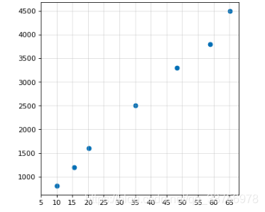 根据上面这些数据,我们预测房屋面积80平米的房租会是多少呢?
首先我们要找到这样房屋面积与价格的映射关系, y=ka+b, 如下图
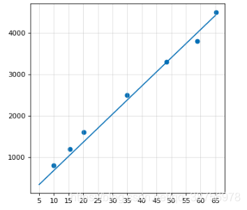
然后通过y=f(x)映射关系,预测房租价格。
这是一个特征值的,那么如果是两个特征值呢?我们找的就是一个平面。

扩展到更多个特征值,我们要找的映射关系就是
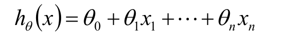
x就是特征值,

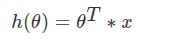
我们可以看做θ。* x。, x。为1,然后j得到这个式子
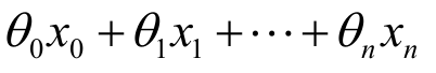
用向量来表示上面这个式子
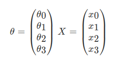
最终我们得到
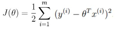
3.误差
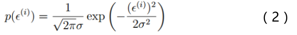
我们得到这个模型,但显然预测值与真实值存在误差,用 ε来表示误差。
对于每个样本则有

由概率论的中心极限定理,可知误差ε是独立并且具有相同的分布,并且服从均值为0方差为σ²的高斯分布。
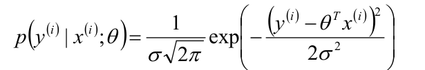
所以
将(1)式带入(2)式
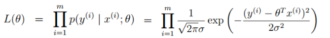
之后用到了似然函数:
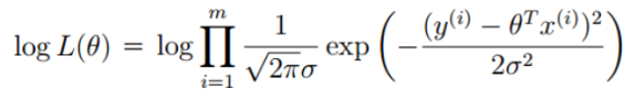
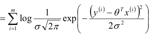
为了便于求解,取对数
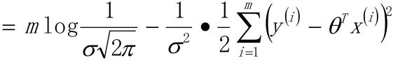
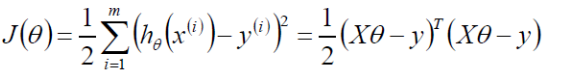
当
最小时, 也就是为0时, logL(θ)值最大,这个式子也就是我们的损失函数。
进一步变换:
然后求它的偏导

令偏导为0,最终可以求得
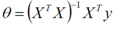
这个就是最小二乘法,也是线性回归损失函数的求解方法之一。
对于上面的房屋面积与房租关系样本的代码示例
import numpy as np
from matplotlib import pyplot as plt
from sklearn.linear_model import LinearRegression as lr


# 房屋面积数据
x_list = [10, 15.5, 20.2, 35.0, 48.3, 58.9, 65.2]
# 对应的房租数据
y_list = [800, 1200, 1600, 2500, 3300, 3800, 4500]

x = np.array(x_list).reshape(-1,1)
y = np.array(y_list).reshape(-1,1)

model = lr()
model.fit(x, y)

y_plot = model.predict(x)

print(model.coef_)

plt.figure(figsize=(5,5),dpi=80, facecolor='w')

plt.scatter(x, y, color='red', linewidths=2,)
plt.plot(x, y_plot, color='blue',)

x_tick = list(range(5, 70, 5))

plt.grid(alpha=0.4)

plt.xticks(x_tick)

plt.show()
结果
[[63.66780288]]

3.波士顿房价预测示例
从sklearn.datasets中获取相关数据集,使用标准线性回归,建立房价预测模型,并绘制房价预测值和真实房价的散点、折线图。
代码示例
# coding:utf-8
from sklearn.datasets import load_boston
from sklearn.linear_model import LinearRegression as lr
from sklearn.model_selection import train_test_split
from sklearn.preprocessing import StandardScaler

from matplotlib import pyplot as plt
from matplotlib import font_manager

font = font_manager.FontProperties(fname="/usr/share/fonts/wps-office/msyhbd.ttf")

def my_predic_fun():
    """
    使用线性回归预测波士顿预测房价
    :return:
    """
    lb = load_boston()

    x_train, x_test, y_train, y_test = train_test_split(lb.data, lb.target, test_size=0.2)

    x_std = StandardScaler()
    y_std = StandardScaler()

    x_train = x_std.fit_transform(x_train)
    x_test = x_std.transform(x_test)
    y_train = y_std.fit_transform(y_train.reshape(-1,1))
    y_test = y_std.transform(y_test.reshape(-1,1))


    model = lr()
    model.fit(x_train, y_train)

    y_predict = y_std.inverse_transform(model.predict(x_test))
    return y_predict, y_std.inverse_transform(y_test)


def draw_fun(y_predict, y_test):
    """
    绘制房价预测与真实值的散点和折线图
    :param y_predict:
    :param y_test:
    :return:
    """
    x = range(1,len(y_predict)+1)
    plt.figure(figsize=(20, 8), dpi=80)
    plt.scatter(x, y_test, label="真实值",color='blue')
    plt.scatter(x, y_predict,label='预测值', color='red')
    plt.plot(x,y_test)
    plt.plot(x,y_predict)

    x_tick = list(x)
    y_tick = list(range(0,60,5))

    plt.legend(prop=font, loc='best')
    plt.xticks(list(x), x_tick)
    plt.yticks(y_tick)
    plt.grid(alpha=0.4)
    plt.show()


if __name__ == '__main__':
    y_predict, y_test = my_predic_fun()
    draw_fun(y_predict, y_test)
结果

参考:https://blog.csdn.net/guoyunfei20/article/details/78053999

 浙公网安备 33010602011771号