PCL 入门教程 - 官方文档翻译
介绍
以下链接描述了一组基本PCL教程。请注意,他们的源代码可能已经作为PCL常规版本的一部分提供,因此在开始复制和粘贴代码之前请检查那里。下面的教程列表是根据git存储库中的reST文件自动生成的。
注意:
在开始阅读之前,请确保您阅读了更高级别的概述文档,网址为http://www.pointclouds.org/documentation/,在“快速入门”下。非常感谢。
一如既往,我们很高兴听到您的意见,并收到您对任何教程的贡献。
基本使用
PCL概览
本教程将引导您了解PCL的组件,提供模块的简短描述,指明模块的位置,并列出不同组件之间的交互关系。
滤波器 Filters
背景:
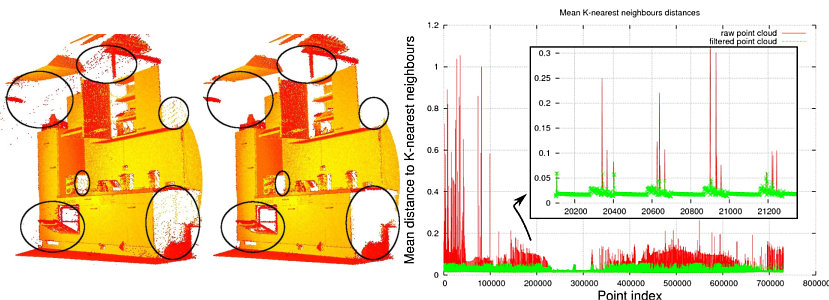
下图给出了噪声去除的示例。由于测量误差,某些数据集存在大量阴影点。这使得本地点云3D特征的估计变得复杂。通过对每个点的邻域进行统计分析,并对不符合特定标准的点进行修剪,可以过滤其中一些异常值。PCL中稀疏离群点消除的实现是基于计算输入数据集中点到邻居距离的分布。对于每个点,计算其到所有相邻点的平均距离。通过假设得到的分布是具有平均值和标准偏差的高斯分布,所有平均距离超出由全局距离平均值和基准偏差定义的区间的点都可以被视为离群值,并从数据集中进行修剪。
文档: http://docs.pointclouds.org/trunk/group__filters.html
示例: http://pointclouds.org/documentation/tutorials/#filtering-tutorial
Interacts with:
    Sample Consensus
    Kdtree
    Octree
安装位置:
    MAC OS X (Homebrew installation)
            Header files: $(PCL_PREFIX)/pcl-$(PCL_VERSION)/pcl/filters/
            Binaries: $(PCL_PREFIX)/bin/
            $(PCL_PREFIX) is the cmake installation prefix CMAKE_INSTALL_PREFIX, e.g., /usr/local/
    Linux
            Header files: $(PCL_PREFIX)/pcl-$(PCL_VERSION)/pcl/filters/
            Binaries: $(PCL_PREFIX)/bin/
            $(PCL_PREFIX) is the cmake installation prefix CMAKE_INSTALL_PREFIX, e.g., /usr/local/
    Windows
            Header files: $(PCL_DIRECTORY)/include/pcl-$(PCL_VERSION)/pcl/filters/
            Binaries: $(PCL_DIRECTORY)/bin/
            $(PCL_DIRECTORY) is the PCL installation directory, e.g., C:\Program Files\PCL $(PCL_VERSION)\
高级使用
特征 Features
3D特征在PCL中的工作方式
在点云中估计曲面法线
曲面法线是几何曲面的重要属性,在许多领域(如计算机图形应用程序)中大量使用,以应用生成着色器和其他视觉效果的正确光源。
给定一个几何曲面,通常很容易将曲面上某个点的法线方向推断为垂直于该点曲面的矢量。然而,由于我们获取的点云数据集代表真实曲面上的一组点样本,因此有两种可能性:
-
使用曲面网格技术,从获取的点云数据集中获取底层曲面,然后从网格中计算曲面法线;
-
使用近似直接从点云数据集推断曲面法线。
本教程将解决后者,即给定点云数据集,直接计算云中每个点的曲面法线。
理论基础
虽然存在许多不同的正常估计方法,但我们将在本教程中集中讨论的方法是最简单的方法之一,公式如下。确定曲面上某一点的法线的问题近似于估算与曲面相切的平面的法线问题,而这又成为一个最小二乘平面拟合估算问题。
因此,估算曲面法线的解决方案简化为分析从查询点最近邻创建的协方差矩阵的特征向量和特征值(或PCA–主成分分析)。更具体地说,对于每个点 pi ,我们将协方差矩阵C组装如下:

其中k是在 pi 邻域中考虑的点邻域的数目, P 表示最近邻域的3D质心, λj 是协方差矩阵的第j个特征值,而 vj 是第j个特征向量。
要从PCL中的一组点估计协方差矩阵,可以使用:
// Placeholder for the 3x3 covariance matrix at each surface patch
Eigen::Matrix3f covariance_matrix;
// 16-bytes aligned placeholder for the XYZ centroid of a surface patch
Eigen::Vector4f xyz_centroid;

// Estimate the XYZ centroid
compute3DCentroid (cloud, xyz_centroid);

// Compute the 3x3 covariance matrix
computeCovarianceMatrix (cloud, xyz_centroid, covariance_matrix);
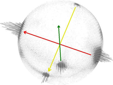
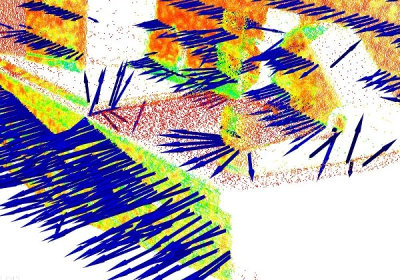
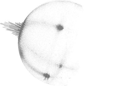
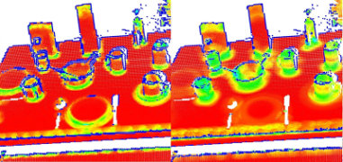
通常,由于没有数学方法来求解法线符号,因此如上所示,通过主成分分析(PCA)计算的法线方向不明确,并且在整个点云数据集上的方向不一致。下图显示了这些对代表厨房环境一部分的较大数据集的两个部分的影响。图的右侧显示了扩展高斯图像(EGI),也称为法线球体,它描述了点云中所有法线的方向。由于数据集为2.5D,因此是从单个视点获取的,因此法线应该只出现在EGI中的一半球体上。然而,由于方向不一致,它们分布在整个球体上。
如果视点vp实际上是已知的,那么这个问题的解决方案是微不足道的。要使所有法线ni始终朝向视点,它们需要满足以下等式:
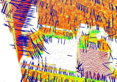
下图显示了上图数据集中的所有法线始终朝向视点后的结果。
要在PCL中手动重新定向给定点法线,可以使用:
flipNormalTowardsViewpoint (const PointT &point, float vp_x, float vp_y, float vp_z, Eigen::Vector4f &normal);
如果数据集有多个采集视点,则上述正常重新定向方法不适用,需要实施更复杂的算法。更多信息,请参见【Rusu论文】。
选择正确的比例
如前所述,需要根据点的周围点邻域支持(也称为k邻域)来估计点处的曲面法线。
最近邻估计问题的细节提出了正确比例因子的问题:给定一个采样点云数据集,在确定点的最近邻集时应该使用的正确k(通过pcl::Feature::setKSearch给定)或r(通过pcl::Feature::setRadiusSearch给定)值是什么?
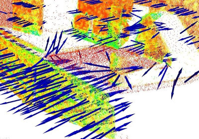
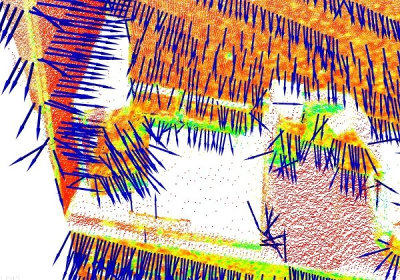
该问题极为重要,并且在点特征表示的自动估计(即,没有用户给定的阈值)中构成了一个限制因素。为了更好地说明这个问题,下图显示了选择较小规模(即,较小的r或k)与选择较大规模(即较大的r或k)的效果。图的左侧描述了一个合理的精心选择的比例因子,估计的曲面法线大致垂直于两个平面,小边在整个表格中都可见。但是,如果比例因子太大(右侧),因此相邻曲面的覆盖点集更大,则估计的点特征表示会扭曲,在两个平面曲面的边上旋转曲面法线,并涂抹边和抑制精细细节。
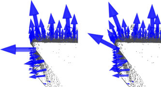
在不深入太多细节的情况下,可以假设目前,必须根据应用程序所需的详细程度选择用于确定点邻域的比例。简单地说,如果杯子把手和圆柱形零件之间边缘的曲率很重要,则比例因子需要足够小以捕捉这些细节,否则需要很大。
估计法线
虽然Features中已经给出了一个正常估计的示例,但为了更好地解释幕后发生的事情,我们将在这里修改其中一个。
以下代码段将估计输入数据集中所有点的一组曲面法线。
#include <pcl/point_types.h>
#include <pcl/features/normal_3d.h>

{
  pcl::PointCloud<pcl::PointXYZ>::Ptr cloud (new pcl::PointCloud<pcl::PointXYZ>);

  ... read, pass in or create a point cloud ...

  // Create the normal estimation class, and pass the input dataset to it
  pcl::NormalEstimation<pcl::PointXYZ, pcl::Normal> ne;
  ne.setInputCloud (cloud);

  // Create an empty kdtree representation, and pass it to the normal estimation object.
  // Its content will be filled inside the object, based on the given input dataset (as no other search surface is given).
  pcl::search::KdTree<pcl::PointXYZ>::Ptr tree (new pcl::search::KdTree<pcl::PointXYZ> ());
  ne.setSearchMethod (tree);

  // Output datasets
  pcl::PointCloud<pcl::Normal>::Ptr cloud_normals (new pcl::PointCloud<pcl::Normal>);

  // Use all neighbors in a sphere of radius 3cm
  ne.setRadiusSearch (0.03);

  // Compute the features
  ne.compute (*cloud_normals);

  // cloud_normals->size () should have the same size as the input cloud->size ()*
}****
NormalEstimation类的实际计算调用在内部没有任何作用,但:
对于点云P中的每一个点p:
  1. 得到p的最近邻
  2. 计算p的曲面法线
  3. 检查n是否始终朝向视点,否则翻转
视点默认为(0,0,0),可以更改为:
setViewPoint (float vpx, float vpy, float vpz);
要计算单点法线,请使用:
computePointNormal (const pcl::PointCloud<PointInT> &cloud, const std::vector<int> &indices, Eigen::Vector4f &plane_parameters, float &curvature);
其中,cloud是包含点的输入点云,index表示来自cloud的k个最近邻居的集合,plane_parameters和curvature表示法线估计的输出,plane_p参数在前3个坐标上保持法线(nx,ny,nz),第四个坐标是D=nc.p_plane(此处为质心)+p。输出曲面曲率估计为协方差矩阵(如上所示)特征值之间的关系,如下所示:
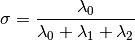
有关该特性的详细描述,请参见M.Pauly、M.Gross和L.P.Kobbelt,“点采样曲面的有效简化”。
使用OpenMP加速正态估计
对于速度敏感的用户,PCL提供了曲面法线估计的附加实现,该实现使用OpenMP的多核/多线程范例来加快计算速度。类的名称是pcl::NormalEstimationOMP,它的API与单线程pcl:∶NormalEssimation 100%兼容,这使得它适合作为一个直接替换。在一个有8个内核的系统上,计算速度应该快6-8倍。
如果您的数据集是有组织的(例如,使用TOF相机、立体相机等获取的,也就是说,它有宽度和高度),要获得更快的结果,请参见使用积分图像的法线估计。
过滤器 Filtering
I/O
关键点 Keypoints
Kd树 KdTree
如何使用Kd树进行搜索
在本教程中,我们将介绍如何使用KdTree查找特定点或位置的K个最近邻,然后我们还将介绍如何查找用户指定半径内的所有临近点(在本例中为随机)。
理论基础
k-d树或k-维树是计算机科学中使用的一种数据结构,用于组织具有k维空间中的一些点。它是一个带有其他约束的二进制搜索树。K-d树对于范围和最近邻搜索非常有用。出于我们的目的,我们通常只处理三维的点云,所以所有的k-d树都是三维的。k-d树的每个级别使用垂直于相应轴的超平面沿特定维度分割所有子级。在树的根处,所有子级都将基于第一个维度进行拆分(即,如果第一个维度坐标小于根,它将位于左子树中,如果大于根,它显然将位于右子树中)。树中的每个级别在下一个维度上进行划分,在其他所有级别都耗尽后返回到第一个维度。构建k-d树的最有效方法是使用一种分区方法,就像快速排序(Quick Sort)用于将中间点放置在根上,以及将较小的一维值放置在左侧,将较大的值放置在右侧。然后在左侧和右侧子树上重复此过程,直到要划分的最后一个树仅由一个元素组成。
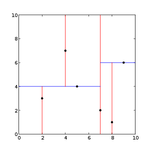
2维Kd树示例
这是最近邻搜索工作原理的演示。
代码
创建一个文件,比方说,kdtree_search。在您喜爱的编辑器中放置cpp,并将以下内容放入其中:
#include <pcl/point_cloud.h>
#include <pcl/kdtree/kdtree_flann.h>

#include <iostream>
#include <vector>
#include <ctime>

int
main ()
{
  srand (time (NULL));

  pcl::PointCloud<pcl::PointXYZ>::Ptr cloud (new pcl::PointCloud<pcl::PointXYZ>);

  // Generate pointcloud data
  cloud->width = 1000;
  cloud->height = 1;
  cloud->points.resize (cloud->width * cloud->height);

  for (std::size_t i = 0; i < cloud->size (); ++i)
  {
    (*cloud)[i].x = 1024.0f * rand () / (RAND_MAX + 1.0f);
    (*cloud)[i].y = 1024.0f * rand () / (RAND_MAX + 1.0f);
    (*cloud)[i].z = 1024.0f * rand () / (RAND_MAX + 1.0f);
  }

  pcl::KdTreeFLANN<pcl::PointXYZ> kdtree;

  kdtree.setInputCloud (cloud);

  pcl::PointXYZ searchPoint;

  searchPoint.x = 1024.0f * rand () / (RAND_MAX + 1.0f);
  searchPoint.y = 1024.0f * rand () / (RAND_MAX + 1.0f);
  searchPoint.z = 1024.0f * rand () / (RAND_MAX + 1.0f);

  // K nearest neighbor search

  int K = 10;

  std::vector<int> pointIdxKNNSearch(K);
  std::vector<float> pointKNNSquaredDistance(K);

  std::cout << "K nearest neighbor search at (" << searchPoint.x
            << " " << searchPoint.y
            << " " << searchPoint.z
            << ") with K=" << K << std::endl;

  if ( kdtree.nearestKSearch (searchPoint, K, pointIdxKNNSearch, pointKNNSquaredDistance) > 0 )
  {
    for (std::size_t i = 0; i < pointIdxKNNSearch.size (); ++i)
      std::cout << "    "  <<   (*cloud)[ pointIdxKNNSearch[i] ].x
                << " " << (*cloud)[ pointIdxKNNSearch[i] ].y
                << " " << (*cloud)[ pointIdxKNNSearch[i] ].z
                << " (squared distance: " << pointKNNSquaredDistance[i] << ")" << std::endl;
  }

  // Neighbors within radius search

  std::vector<int> pointIdxRadiusSearch;
  std::vector<float> pointRadiusSquaredDistance;

  float radius = 256.0f * rand () / (RAND_MAX + 1.0f);

  std::cout << "Neighbors within radius search at (" << searchPoint.x
            << " " << searchPoint.y
            << " " << searchPoint.z
            << ") with radius=" << radius << std::endl;


  if ( kdtree.radiusSearch (searchPoint, radius, pointIdxRadiusSearch, pointRadiusSquaredDistance) > 0 )
  {
    for (std::size_t i = 0; i < pointIdxRadiusSearch.size (); ++i)
      std::cout << "    "  <<   (*cloud)[ pointIdxRadiusSearch[i] ].x
                << " " << (*cloud)[ pointIdxRadiusSearch[i] ].y
                << " " << (*cloud)[ pointIdxRadiusSearch[i] ].z
                << " (squared distance: " << pointRadiusSquaredDistance[i] << ")" << std::endl;
  }


  return 0;
}
解释
以下代码首先用系统时间播种rand(),然后用随机数据创建并填充PointCloud。
  srand (time (NULL));

  pcl::PointCloud<pcl::PointXYZ>::Ptr cloud (new pcl::PointCloud<pcl::PointXYZ>);

  // Generate pointcloud data
  cloud->width = 1000;
  cloud->height = 1;
  cloud->points.resize (cloud->width * cloud->height);

  for (std::size_t i = 0; i < cloud->size (); ++i)
  {
    (*cloud)[i].x = 1024.0f * rand () / (RAND_MAX + 1.0f);
    (*cloud)[i].y = 1024.0f * rand () / (RAND_MAX + 1.0f);
    (*cloud)[i].z = 1024.0f * rand () / (RAND_MAX + 1.0f);
  }
接下来的代码创建kdtree对象,并将随机创建的云设置为输入。然后我们创建一个“searchPoint”,它被分配了随机坐标。
  pcl::KdTreeFLANN<pcl::PointXYZ> kdtree;

  kdtree.setInputCloud (cloud);

  pcl::PointXYZ searchPoint;

  searchPoint.x = 1024.0f * rand () / (RAND_MAX + 1.0f);
  searchPoint.y = 1024.0f * rand () / (RAND_MAX + 1.0f);
  searchPoint.z = 1024.0f * rand () / (RAND_MAX + 1.0f);
现在我们创建一个整数(并将其设置为10)和两个向量,用于存储搜索中的K个最近邻居。
  // K nearest neighbor search

  int K = 10;

  std::vector<int> pointIdxKNNSearch(K);
  std::vector<float> pointKNNSquaredDistance(K);

  std::cout << "K nearest neighbor search at (" << searchPoint.x
            << " " << searchPoint.y
            << " " << searchPoint.z
            << ") with K=" << K << std::endl;
假设我们的KdTree返回的最近邻不为零,它会打印出随机“searchPoint”的所有10个最近邻的位置,这些位置存储在我们之前创建的向量中。
  if ( kdtree.nearestKSearch (searchPoint, K, pointIdxKNNSearch, pointKNNSquaredDistance) > 0 )
  {
    for (std::size_t i = 0; i < pointIdxKNNSearch.size (); ++i)
      std::cout << "    "  <<   (*cloud)[ pointIdxKNNSearch[i] ].x
                << " " << (*cloud)[ pointIdxKNNSearch[i] ].y
                << " " << (*cloud)[ pointIdxKNNSearch[i] ].z
                << " (squared distance: " << pointKNNSquaredDistance[i] << ")" << std::endl;
  }
现在,我们的代码演示了如何在某些(随机生成的)半径内找到给定“searchPoint”的所有邻居。它再次创建了两个向量来存储邻居的信息。
  // Neighbors within radius search

  std::vector<int> pointIdxRadiusSearch;
  std::vector<float> pointRadiusSquaredDistance;

  float radius = 256.0f * rand () / (RAND_MAX + 1.0f);
同样,就像之前一样,如果KdTree在指定半径内返回0个以上的邻居,它会打印出存储在向量中的这些点的坐标。
  if ( kdtree.radiusSearch (searchPoint, radius, pointIdxRadiusSearch, pointRadiusSquaredDistance) > 0 )
  {
    for (std::size_t i = 0; i < pointIdxRadiusSearch.size (); ++i)
      std::cout << "    "  <<   (*cloud)[ pointIdxRadiusSearch[i] ].x
                << " " << (*cloud)[ pointIdxRadiusSearch[i] ].y
                << " " << (*cloud)[ pointIdxRadiusSearch[i] ].z
                << " (squared distance: " << pointRadiusSquaredDistance[i] << ")" << std::endl;
  }
编译和运行程序
将以下行添加到CMakeLists.txt文件:
cmake_minimum_required(VERSION 3.5 FATAL_ERROR)

project(kdtree_search)

find_package(PCL 1.2 REQUIRED)

include_directories(${PCL_INCLUDE_DIRS})
link_directories(${PCL_LIBRARY_DIRS})
add_definitions(${PCL_DEFINITIONS})

add_executable (kdtree_search kdtree_search.cpp)
target_link_libraries (kdtree_search ${PCL_LIBRARIES})
创建可执行文件后,可以运行它。只需做:
$ ./kdtree_search
运行之后,您应该会看到类似的内容:
K nearest neighbor search at (455.807 417.256 406.502) with K=10
  494.728 371.875 351.687 (squared distance: 6578.99)
  506.066 420.079 478.278 (squared distance: 7685.67)
  368.546 427.623 416.388 (squared distance: 7819.75)
  474.832 383.041 323.293 (squared distance: 8456.34)
  470.992 334.084 468.459 (squared distance: 10986.9)
  560.884 417.637 364.518 (squared distance: 12803.8)
  466.703 475.716 306.269 (squared distance: 13582.9)
  456.907 336.035 304.529 (squared distance: 16996.7)
  452.288 387.943 279.481 (squared distance: 17005.9)
  476.642 410.422 268.057 (squared distance: 19647.9)
Neighbors within radius search at (455.807 417.256 406.502) with radius=225.932
  494.728 371.875 351.687 (squared distance: 6578.99)
  506.066 420.079 478.278 (squared distance: 7685.67)
  368.546 427.623 416.388 (squared distance: 7819.75)
  474.832 383.041 323.293 (squared distance: 8456.34)
  470.992 334.084 468.459 (squared distance: 10986.9)
  560.884 417.637 364.518 (squared distance: 12803.8)
  466.703 475.716 306.269 (squared distance: 13582.9)
  456.907 336.035 304.529 (squared distance: 16996.7)
  452.288 387.943 279.481 (squared distance: 17005.9)
  476.642 410.422 268.057 (squared distance: 19647.9)
  499.429 541.532 351.35 (squared distance: 20389)
  574.418 452.961 334.7 (squared distance: 20498.9)
  336.785 391.057 488.71 (squared distance: 21611)
  319.765 406.187 350.955 (squared distance: 21715.6)
  528.89 289.583 378.979 (squared distance: 22399.1)
  504.509 459.609 541.732 (squared distance: 22452.8)
  539.854 349.333 300.395 (squared distance: 22936.3)
  548.51 458.035 292.812 (squared distance: 23182.1)
  546.284 426.67 535.989 (squared distance: 25041.6)
  577.058 390.276 508.597 (squared distance: 25853.1)
  543.16 458.727 276.859 (squared distance: 26157.5)
  613.997 387.397 443.207 (squared distance: 27262.7)
  608.235 467.363 327.264 (squared distance: 32023.6)
  506.842 591.736 391.923 (squared distance: 33260.3)
  529.842 475.715 241.532 (squared distance: 36113.7)
  485.822 322.623 244.347 (squared distance: 36150.5)
  362.036 318.014 269.201 (squared distance: 37493.6)
  493.806 600.083 462.742 (squared distance: 38032.3)
  392.315 368.085 585.37 (squared distance: 38442.9)
  303.826 428.659 533.642 (squared distance: 39392.8)
  616.492 424.551 289.524 (squared distance: 39556.8)
  320.563 333.216 278.242 (squared distance: 41804.5)
  646.599 502.256 424.46 (squared distance: 43948.8)
  556.202 325.013 568.252 (squared distance: 44751)
  291.27 497.352 515.938 (squared distance: 45463.9)
  286.483 322.401 495.377 (squared distance: 45567.2)
  367.288 550.421 550.551 (squared distance: 46318.6)
  595.122 582.77 394.894 (squared distance: 46938.1)
  256.784 499.401 379.931 (squared distance: 47064.1)
  430.782 230.854 293.829 (squared distance: 48067.2)
  261.051 486.593 329.854 (squared distance: 48612.7)
  602.061 327.892 545.269 (squared distance: 48632.4)
  347.074 610.994 395.622 (squared distance: 49475.6)
  482.876 284.894 583.888 (squared distance: 49718.6)
  356.962 247.285 514.959 (squared distance: 50423.7)
  282.065 509.488 516.216 (squared distance: 50730.4)
