3-3高阶API示范
Pytorch没有官方的高阶API,一般需要用户自己实现训练循环、验证循环和预测循环。
坐着通过仿照Keras的功能对Pytorch的nn.Module进行了封装,设计了torchkeras.KerasModel类
实现了fit,evaluate等方法,相当于用户自定义高阶API。
并示范了用它实现线性回归和DNN二分类模型。
torchkeras.KerasModel类看起来非常强大,但实际上它们的源码非常简单,不足200行。我们在第一章中用到的代码其实就是torchkeras库的核心源码。
import torch
import torchkeras


print("torch.__version__="+torch.__version__)
print("torchkeras.__version__="+torchkeras.__version__)
1.线性回归模型
import numpy as np
import pandas as pd
import matplotlib.pyplot as plt
import torch
from torch import nn
import torch.nn.functional as F
from torch.utils.data import Dataset, DataLoader, TensorDataset
#样本数量
n = 400
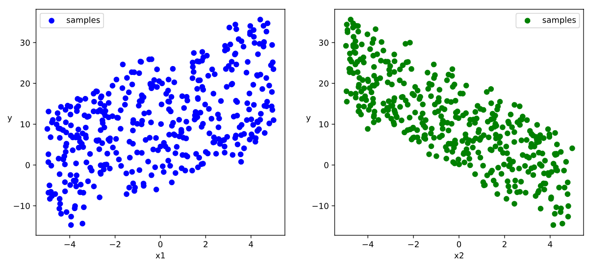
# 生成测试用数据集
X = 10*torch.rand([n,2])-5.0 #torch.rand是均匀分布
w0 = torch.tensor([[2.0],[-3.0]])
b0 = torch.tensor([[10.0]])
Y = X@w0 + b0 + torch.normal( 0.0,2.0,size = [n,1]) # @表示矩阵乘法,增加正态扰动
# 数据可视化
%matplotlib inline
%config InlineBackend.figure_format = 'svg'
plt.figure(figsize = (12,5))
ax1 = plt.subplot(121)
ax1.scatter(X[:,0],Y[:,0], c = "b",label = "samples")
ax1.legend()
plt.xlabel("x1")
plt.ylabel("y",rotation = 0)
ax2 = plt.subplot(122)
ax2.scatter(X[:,1],Y[:,0], c = "g",label = "samples")
ax2.legend()
plt.xlabel("x2")
plt.ylabel("y",rotation = 0)
plt.show()
# 构建输入数据管道
ds = TensorDataset(X, Y)
ds_train, ds_val = torch.utils.data.random_split(ds, [int(400*0.7), 400-int(400*0.7)])
dl_train = DataLoader(ds_train, batch_size=16, shuffle=True, num_workers=2)
dl_val = DataLoader(ds_val, batch_size=16, num_workers=2)

features, labels = next(iter(dl_train))
# 定义模型
class LinearRegression(nn.Module):
def __init__(self):
super().__init__()
self.fc = nn.Linear(2, 1)
def forward(self, x):
return self.fc(x)
net = LinearRegression()
from torchkeras import summary
print(summary(net, input_data=features))
"""
--------------------------------------------------------------------------
Layer (type) Output Shape Param #
==========================================================================
Linear-1 [-1, 1] 3
==========================================================================
Total params: 3
Trainable params: 3
Non-trainable params: 0
--------------------------------------------------------------------------
Input size (MB): 0.000076
Forward/backward pass size (MB): 0.000008
Params size (MB): 0.000011
Estimated Total Size (MB): 0.000095
--------------------------------------------------------------------------
"""
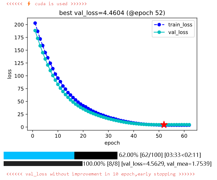
# 训练模型
from torchkeras import KerasModel
import torchmetrics
net = LinearRegression()
model = KerasModel(net=net,
loss_fn=nn.MSELoss(),
metrics_dict={'mea': torchmetrics.MeanAbsoluteError()},
optimizer=torch.optim.Adam(net.parameters(), lr=0.01))
df_history = model.fit(train_data=dl_train,
val_data=dl_val,
epochs=100,
ckpt_path='checkpoint',
patience=10,
monitor='val_loss',
mode='min')
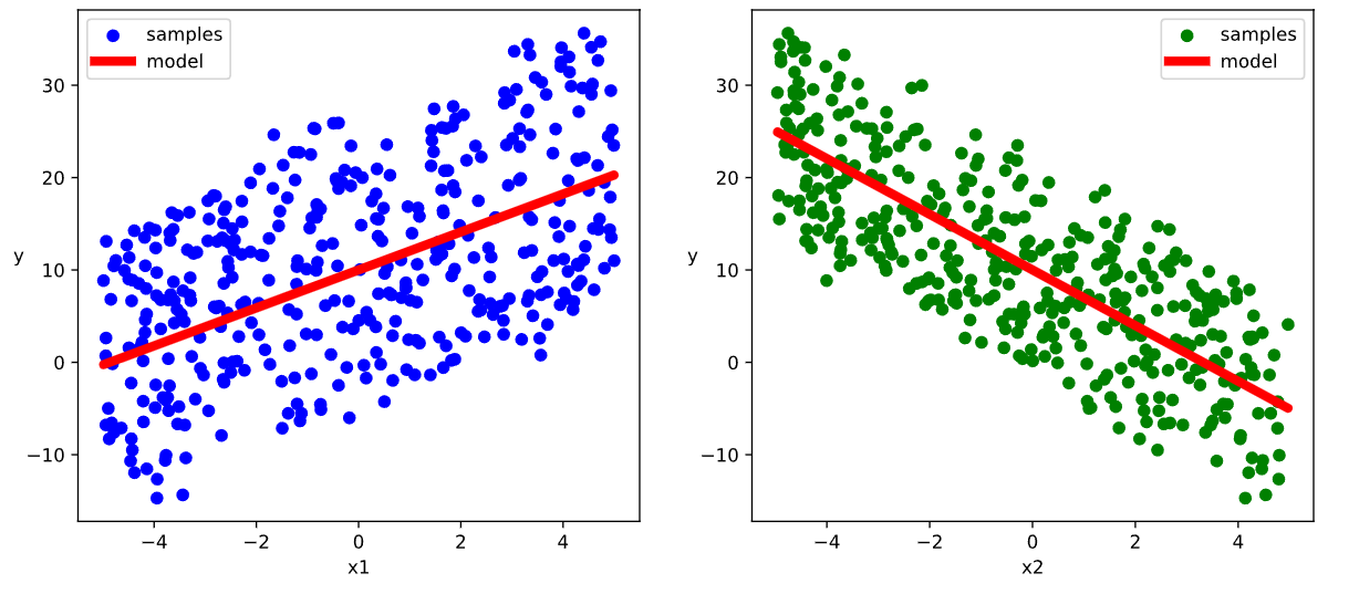
# 结果可视化

%matplotlib inline
%config InlineBackend.figure_format = 'svg'

w,b = net.state_dict()["fc.weight"],net.state_dict()["fc.bias"]

plt.figure(figsize = (12,5))
ax1 = plt.subplot(121)
ax1.scatter(X[:,0],Y[:,0], c = "b",label = "samples")
ax1.plot(X[:,0],w[0,0]*X[:,0]+b[0],"-r",linewidth = 5.0,label = "model")
ax1.legend()
plt.xlabel("x1")
plt.ylabel("y",rotation = 0)


ax2 = plt.subplot(122)
ax2.scatter(X[:,1],Y[:,0], c = "g",label = "samples")
ax2.plot(X[:,1],w[0,1]*X[:,1]+b[0],"-r",linewidth = 5.0,label = "model")
ax2.legend()
plt.xlabel("x2")
plt.ylabel("y",rotation = 0)

plt.show()
# 评估模型
df_history.tail()

"""
	epoch	train_loss	train_mea	lr	val_loss	val_mea
57	58	3.677166	1.493061	0.01	4.539605	1.755498
58	59	3.654148	1.495321	0.01	4.620949	1.772233
59	60	3.715624	1.500220	0.01	4.598151	1.764618
60	61	3.663024	1.490255	0.01	4.571722	1.757480
61	62	3.839647	1.488007	0.01	4.562901	1.753924
"""

model.evaluate(dl_val)
"""
{'val_loss': 4.460375756025314, 'val_mea': 1.7544724941253662}
"""

# 使用模型
dl = DataLoader(TensorDataset(X))

result = []
with torch.no_grad():
    for batch in dl:
        features = batch[0].to(model.accelerator.device)
        res = net(features)
        result.extend(res.tolist())

result = np.array(result).flatten()
print(result[:10])
"""
[-4.31195259  4.58132076 12.62739372 -0.60054398  6.42537785 -2.99616528
  8.89183521  5.3079319  -7.17126656 15.40559959]
"""
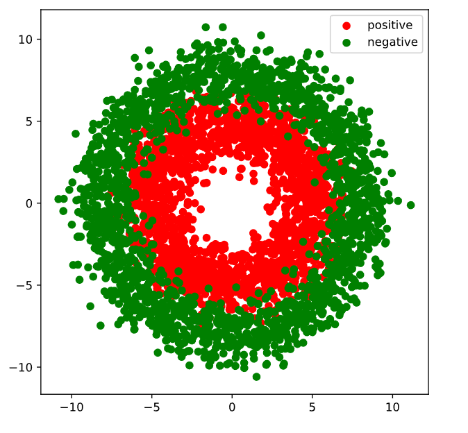
2.DNN二分类模型
# 准备数据
import numpy as np
import pandas as pd
from matplotlib import pyplot as plt
import torch
from torch import nn
import torch.nn.functional as F
from torch.utils.data import Dataset,DataLoader,TensorDataset
import torchkeras
import pytorch_lightning as pl
%matplotlib inline
%config InlineBackend.figure_format = 'svg'

#正负样本数量
n_positive,n_negative = 2000,2000

#生成正样本, 小圆环分布
r_p = 5.0 + torch.normal(0.0,1.0,size = [n_positive,1])
theta_p = 2*np.pi*torch.rand([n_positive,1])
Xp = torch.cat([r_p*torch.cos(theta_p),r_p*torch.sin(theta_p)],axis = 1)
Yp = torch.ones_like(r_p)

#生成负样本, 大圆环分布
r_n = 8.0 + torch.normal(0.0,1.0,size = [n_negative,1])
theta_n = 2*np.pi*torch.rand([n_negative,1])
Xn = torch.cat([r_n*torch.cos(theta_n),r_n*torch.sin(theta_n)],axis = 1)
Yn = torch.zeros_like(r_n)

#汇总样本
X = torch.cat([Xp,Xn],axis = 0)
Y = torch.cat([Yp,Yn],axis = 0)


#可视化
plt.figure(figsize = (6,6))
plt.scatter(Xp[:,0],Xp[:,1],c = "r")
plt.scatter(Xn[:,0],Xn[:,1],c = "g")
plt.legend(["positive","negative"]);
# 构建数据管道
ds = TensorDataset(X,Y)

ds_train,ds_val = torch.utils.data.random_split(ds,[int(len(ds)*0.7),len(ds)-int(len(ds)*0.7)])
dl_train = DataLoader(ds_train,batch_size = 100,shuffle=True,num_workers=2)
dl_val = DataLoader(ds_val,batch_size = 100,num_workers=2)

for features,labels in dl_train:
    break
# 定义模型
class Net(nn.Module):
    def __init__(self):
        super().__init__()
        self.fc1 = nn.Linear(2, 4)
        self.fc2 = nn.Linear(4, 8)
        self.fc3 = nn.Linear(8, 1)

    def forward(self, x):
        x = F.relu(self.fc1(x))
        x = F.relu(self.fc2(x))
        y = self.fc3(x)
        return y
from torchkeras import KerasModel
from torchkeras.metrics import Accuracy
net = Net()
loss_fn = nn.BCEWithLogitsLoss()
metric_dict = {'acc': Accuracy()}
optimizer = torch.optim.Adam(net.parameters(), lr=0.001)
model = KerasModel(net,
loss_fn=loss_fn,
metrics_dict=metric_dict,
optimizer=optimizer)
from torchkeras import summary
print(summary(net, input_data=features))
"""
--------------------------------------------------------------------------
Layer (type) Output Shape Param #
==========================================================================
Linear-1 [-1, 4] 12
Linear-2 [-1, 8] 40
Linear-3 [-1, 1] 9
==========================================================================
Total params: 61
Trainable params: 61
Non-trainable params: 0
--------------------------------------------------------------------------
Input size (MB): 0.000076
Forward/backward pass size (MB): 0.000099
Params size (MB): 0.000233
Estimated Total Size (MB): 0.000408
--------------------------------------------------------------------------
"""
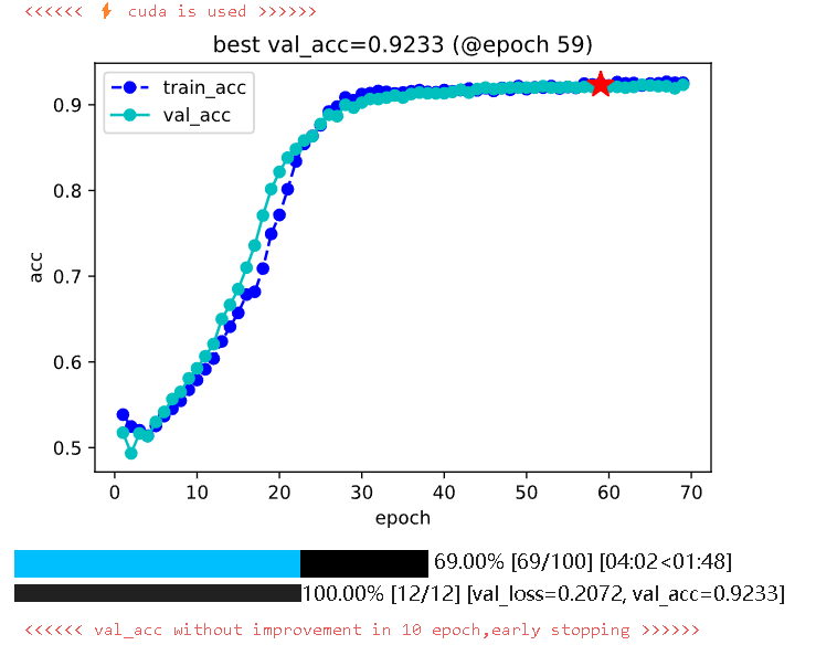
# 训练模型
df_history = model.fit(
train_data=dl_train,
val_data=dl_val,
epochs=100,
ckpt_path='checkpoint',
patience=10,
monitor='val_acc',
mode='max'
)
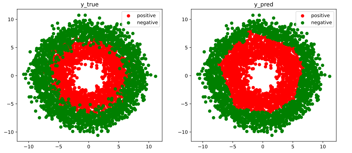
# 结果可视化
fig, (ax1,ax2) = plt.subplots(nrows=1,ncols=2,figsize = (12,5))
ax1.scatter(Xp[:,0],Xp[:,1], c="r")
ax1.scatter(Xn[:,0],Xn[:,1],c = "g")
ax1.legend(["positive","negative"]);
ax1.set_title("y_true");

Xp_pred = X[torch.squeeze(net.forward(X)>=0.5)]
Xn_pred = X[torch.squeeze(net.forward(X)<0.5)]

ax2.scatter(Xp_pred[:,0],Xp_pred[:,1],c = "r")
ax2.scatter(Xn_pred[:,0],Xn_pred[:,1],c = "g")
ax2.legend(["positive","negative"]);
ax2.set_title("y_pred");
model.evaluate(dl_val)
"""
{'val_loss': 0.21838669975598654, 'val_acc': 0.9233333468437195}
"""

# 使用模型
device = model.accelerator.device
@torch.no_grad()
def predict(net, dl):
    net.eval()
    result = torch.cat([net.forward(t[0].to(device)) for t in dl])
    return result.data

predictions = F.sigmoid(predict(net, dl_val)[:10])

predictions
"""
tensor([[0.0090],
        [0.0220],
        [0.0051],
        [0.2869],
        [0.3830],
        [0.0024],
        [0.9632],
        [0.9817],
        [0.9072],
        [0.1991]], device='cuda:0')
"""
作者:lotuslaw
出处:https://www.cnblogs.com/lotuslaw/p/18057708
版权:本作品采用「署名-非商业性使用-相同方式共享 4.0 国际」许可协议进行许可。
标签:
Pytorch


【推荐】国内首个AI IDE,深度理解中文开发场景,立即下载体验Trae
【推荐】编程新体验,更懂你的AI,立即体验豆包MarsCode编程助手
【推荐】抖音旗下AI助手豆包,你的智能百科全书,全免费不限次数
【推荐】轻量又高性能的 SSH 工具 IShell:AI 加持,快人一步
· 阿里最新开源QwQ-32B,效果媲美deepseek-r1满血版,部署成本又又又降低了!
· 开源Multi-agent AI智能体框架aevatar.ai,欢迎大家贡献代码
· Manus重磅发布:全球首款通用AI代理技术深度解析与实战指南
· 被坑几百块钱后,我竟然真的恢复了删除的微信聊天记录!
· 没有Manus邀请码?试试免邀请码的MGX或者开源的OpenManus吧