3-1低阶API示范
- 下面的范例使用Pytorch的低阶API实现线性回归和DNN二分类
- 低阶API主要包括张量操作,计算图和自动微分
import os
import datetime

# 打印时间
def printbar():
    nowtime = datetime.datetime.now().strftime('%Y-%m-%d %H:%M:%S')
    print('\n' + '========='*8 + '%s' % nowtime)

#mac系统上pytorch和matplotlib在jupyter中同时跑需要更改环境变量
# os.environ["KMP_DUPLICATE_LIB_OK"]="TRUE"

import torch
print('torch.__version__=' + torch.__version__)

"""
torch.__version__=2.1.1+cu118
"""
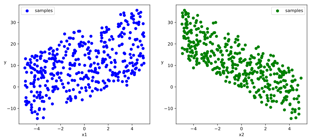
1.线性回归模型
# 准备数据
import numpy as np
import pandas as pd
import matplotlib.pyplot as plt
import torch
from torch import nn

# 样本数量
n = 400

# 生成测试用数据集
X = 10*torch.rand([n, 2]) - 5.0  # torch.rand是均匀分布
w0 = torch.tensor([[2.0], [-3.0]])
b0 = torch.tensor([[10.0]])
Y = X@w0 + b0 + torch.normal(0.0, 2.0, size=[n, 1])

# 数据可视化
%matplotlib inline
%config InlineBackend.figure_format='svg'

plt.figure(figsize=(12, 5))
ax1 = plt.subplot(121)
ax1.scatter(X[:, 0].numpy(), Y[:, 0].numpy(), c='b', label='samples')
ax1.legend()
plt.xlabel('x1')
plt.ylabel('y', rotation=0)

ax2 = plt.subplot(122)
ax2.scatter(X[:,1].numpy(),Y[:,0].numpy(), c = "g",label = "samples")
ax2.legend()
plt.xlabel("x2")
plt.ylabel("y",rotation = 0)
plt.show()
# 构建数据管道迭代器
def data_iter(features, labels, batch_size=8):
    num_examples = len(features)
    indices = list(range(num_examples))
    np.random.shuffle(indices)
    for i in range(0, num_examples, batch_size):
        indexs = torch.LongTensor(indices[i: min(i+batch_size, num_examples)])
        yield features.index_select(0, indexs), labels.index_select(0, indexs)

# 测试数据管道效果
batch_size = 8
features, labels = next(data_iter(X, Y, batch_size))
print(features)
print(labels)

"""
tensor([[ 0.5934,  0.2840],
        [ 4.5548, -4.5195],
        [ 0.1557,  1.7895],
        [-3.6943, -3.1508],
        [-4.4599,  3.5827],
        [ 4.3526,  3.9085],
        [ 4.6064,  4.2197],
        [-3.9680,  3.2592]])
tensor([[  7.5161],
        [ 29.0174],
        [  5.4269],
        [ 14.0158],
        [-10.6806],
        [  8.7862],
        [  7.8535],
        [ -2.4455]])
"""
class LinearRegression:
    def __init__(self):
        self.w = torch.randn_like(w0, requires_grad=True)
        self.b = torch.zeros_like(b0, requires_grad=True)

    # 正向传播
    def forward(self, x):
        return x@self.w + self.b

    # 损失函数'
    def loss_fn(self, y_pred, y_true):
        return torch.mean((y_pred - y_true) ** 2 / 2)

model = LinearRegression()

def train_step(model, features, labels):
    predictions = model.forward(features)
    loss = model.loss_fn(predictions, labels)

    # 反向传播求梯度
    loss.backward()

    # 使用torch.no_grad()避免梯度记录,也可以通过操作model.w.data实现避免梯度记录
    with torch.no_grad():
        model.w -= 0.001 * model.w.grad
        model.b -= 0.001 * model.b.grad

        # 梯度清零
        model.w.grad.zero_()
        model.b.grad.zero_()
    return loss

# 测试train_step效果
batch_size = 10
features, labels = next(data_iter(X, Y, batch_size))
train_step(model, features, labels)
"""
tensor(128.2067, grad_fn=<MeanBackward0>)
"""

def train_model(model, epochs):
    for epoch in range(1, epochs+1):
        for features, labels in data_iter(X, Y, 10):
            loss = train_step(model, features, labels)

        if epoch % 20 == 0:
            printbar()
            print('epoch =', epoch, 'loss = ', loss.item())
            print('model.w =', model.w.data)
            print('model.b = ', model.b.data)
train_model(model, epochs=200)
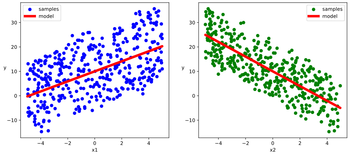
# 结果可视化
%matplotlib inline
%config InlineBackend.figure_format='svg'


plt.figure(figsize = (12,5))
ax1 = plt.subplot(121)
ax1.scatter(X[:,0].numpy(),Y[:,0].numpy(), c = "b",label = "samples")
ax1.plot(X[:,0].numpy(),(model.w[0].data*X[:,0]+model.b[0].data).numpy(),"-r",linewidth = 5.0,label = "model")
ax1.legend()
plt.xlabel("x1")
plt.ylabel("y",rotation = 0)


ax2 = plt.subplot(122)
ax2.scatter(X[:,1].numpy(),Y[:,0].numpy(), c = "g",label = "samples")
ax2.plot(X[:,1].numpy(),(model.w[1].data*X[:,1]+model.b[0].data).numpy(),"-r",linewidth = 5.0,label = "model")
ax2.legend()
plt.xlabel("x2")
plt.ylabel("y",rotation = 0)

plt.show()
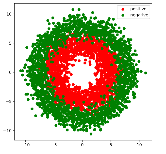
2.DNN二分类模型
# 准备数据
import numpy as np
import pandas as pd
import matplotlib.pyplot as plt
import torch
%matplotlib inline
%config InlineBackend.figure_format='svg'

#正负样本数量
n_positive,n_negative = 2000,2000

#生成正样本, 小圆环分布
r_p = 5.0 + torch.normal(0.0,1.0,size = [n_positive,1])
theta_p = 2*np.pi*torch.rand([n_positive,1])
Xp = torch.cat([r_p*torch.cos(theta_p),r_p*torch.sin(theta_p)],axis = 1)

#生成负样本, 大圆环分布
r_n = 8.0 + torch.normal(0.0,1.0,size = [n_negative,1])
theta_n = 2*np.pi*torch.rand([n_negative,1])
Xn = torch.cat([r_n*torch.cos(theta_n),r_n*torch.sin(theta_n)],axis = 1)

#汇总样本
X = torch.cat([Xp,Xn],axis = 0)

#可视化
plt.figure(figsize = (6,6))
plt.scatter(Xp[:,0].numpy(),Xp[:,1].numpy(),c = "r")
plt.scatter(Xn[:,0].numpy(),Xn[:,1].numpy(),c = "g")
plt.legend(["positive","negative"]);
# 构建数据管道迭代器
def data_iter(features, labels, batch_size=8):
    num_examples = len(features)
    indices = list(range(num_examples))
    np.random.shuffle(indices)  #样本的读取顺序是随机的
    for i in range(0, num_examples, batch_size):
        indexs = torch.LongTensor(indices[i: min(i + batch_size, num_examples)])
        yield  features.index_select(0, indexs), labels.index_select(0, indexs)

# 测试数据管道效果
batch_size = 8
(features,labels) = next(data_iter(X,Y,batch_size))
print(features)
print(labels)

"""
tensor([[ 2.0455, -8.4665],
        [-4.2541, -2.2007],
        [ 1.3186, -4.0994],
        [ 1.1789, -6.0809],
        [ 3.2550, -2.1135],
        [-7.4584, -2.3193],
        [-2.2631,  7.4502],
        [-6.7228,  5.1542]])
tensor([[0.],
        [1.],
        [1.],
        [0.],
        [1.],
        [0.],
        [0.],
        [0.]])
"""
class DNNModel(torch.nn.Module):
    def __init__(self):
        super().__init__()
        self.w1 = torch.nn.Parameter(torch.randn(2, 4))
        self.b1 = torch.nn.Parameter(torch.zeros(1, 4))
        self.w2 = torch.nn.Parameter(torch.randn(4, 8))
        self.b2 = torch.nn.Parameter(torch.zeros(1, 8))
        self.w3 = torch.nn.Parameter(torch.randn(8, 1))
        self.b3 = torch.nn.Parameter(torch.zeros(1, 1))

    def forward(self, x):
        x = torch.relu(x@self.w1 + self.b1)
        x = torch.relu(x@self.w2 + self.b2)
        y = torch.sigmoid(x@self.w3 + self.b3)
        return y

    def loss_fn(self, y_pred, y_true):
        eps = 1e-7
        y_pred = torch.clamp(y_pred, eps, 1.0-eps)
        bce = -y_true*torch.log(y_pred) - (1-y_true)*torch.log(1-y_pred)
        return torch.mean(bce)

    def metric_fn(self, y_pred, y_true):
        y_pred = torch.where(y_pred > 0.5, torch.ones_like(y_pred, dtype=torch.float32),
                            torch.zeros_like(y_pred, dtype=torch.float32))
        acc = torch.mean(1-torch.abs(y_true - y_pred))
        return acc

model = DNNModel()

# 测试模型结构
batch_size = 10
(features,labels) = next(data_iter(X,Y,batch_size))

predictions = model(features)

loss = model.loss_fn(labels,predictions)
metric = model.metric_fn(labels,predictions)

print("init loss:", loss.item())
print("init metric:", metric.item())
"""
init loss: 8.984026908874512
init metric: 0.4419798254966736
"""
def train_step(model, features, labels):
# 正向传播求损失
predictions = model.forward(features)
loss = model.loss_fn(predictions,labels)
metric = model.metric_fn(predictions,labels)
# 反向传播求梯度
loss.backward()
# 梯度下降法更新参数
for param in model.parameters():
#注意是对param.data进行重新赋值,避免此处操作引起梯度记录
param.data = (param.data - 0.01*param.grad.data)
# 梯度清零
model.zero_grad()
return loss.item(),metric.item()
def train_model(model,epochs):
for epoch in range(1,epochs+1):
loss_list,metric_list = [],[]
for features, labels in data_iter(X,Y,20):
lossi,metrici = train_step(model,features,labels)
loss_list.append(lossi)
metric_list.append(metrici)
loss = np.mean(loss_list)
metric = np.mean(metric_list)
if epoch%10==0:
printbar()
print("epoch =",epoch,"loss = ",loss,"metric = ",metric)
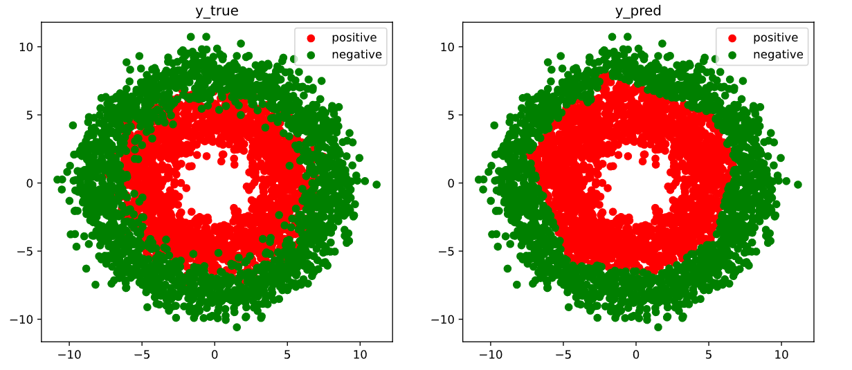
train_model(model,epochs = 100)
# 结果可视化
fig, (ax1,ax2) = plt.subplots(nrows=1,ncols=2,figsize = (12,5))
ax1.scatter(Xp[:,0],Xp[:,1], c="r")
ax1.scatter(Xn[:,0],Xn[:,1],c = "g")
ax1.legend(["positive","negative"]);
ax1.set_title("y_true");
Xp_pred = X[torch.squeeze(model.forward(X)>=0.5)]
Xn_pred = X[torch.squeeze(model.forward(X)<0.5)]
ax2.scatter(Xp_pred[:,0],Xp_pred[:,1],c = "r")
ax2.scatter(Xn_pred[:,0],Xn_pred[:,1],c = "g")
ax2.legend(["positive","negative"]);
ax2.set_title("y_pred");
作者:lotuslaw
出处:https://www.cnblogs.com/lotuslaw/p/18052914
版权:本作品采用「署名-非商业性使用-相同方式共享 4.0 国际」许可协议进行许可。
标签:
Pytorch


【推荐】国内首个AI IDE,深度理解中文开发场景,立即下载体验Trae
【推荐】编程新体验,更懂你的AI,立即体验豆包MarsCode编程助手
【推荐】抖音旗下AI助手豆包,你的智能百科全书,全免费不限次数
【推荐】轻量又高性能的 SSH 工具 IShell:AI 加持,快人一步
· 阿里最新开源QwQ-32B,效果媲美deepseek-r1满血版,部署成本又又又降低了!
· 开源Multi-agent AI智能体框架aevatar.ai,欢迎大家贡献代码
· Manus重磅发布:全球首款通用AI代理技术深度解析与实战指南
· 被坑几百块钱后,我竟然真的恢复了删除的微信聊天记录!
· 没有Manus邀请码?试试免邀请码的MGX或者开源的OpenManus吧
2021-03-04 6-数据加载&Pandas绘图&Scipy初步
2021-03-04 5-Pandas数据处理