3-1低阶API示例——eat_tensorflow2_in_30_days
3-1低阶API示范#
下面的范例使用TensorFlow的低阶API实现线性回归模型和DNN二分类模型
低阶API主要包括张量操作,计算图和自动微分
import tensorflow as tf

# 打印时间分割线
@tf.function
def printbar():
    today_ts = tf.timestamp() % (24*60*60)
    hour = tf.cast(today_ts//3600+8, tf.int32) % tf.constant(24)
    minite = tf.cast((today_ts%3600) // 60, tf.int32)
    second = tf.cast(tf.floor(today_ts % 60), tf.int32)

    def timeformat(m):
        if tf.strings.length(tf.strings.format('{}', m)) == 1:
            return tf.strings.format('0{}', m)
        else:
            return tf.strings.format('{}', m)

    timestring = tf.strings.join([timeformat(hour), timeformat(minit), timeformat(second)], separator=':')
    tf.print('=========='*8 + timestring)
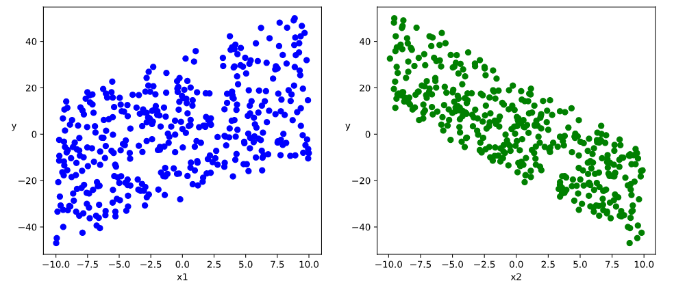
线性回归模型#
- 准备数据
import numpy as np
import pandas as pd
import matplotlib.pyplot as plt
import tensorflow as tf

# 样本数量
n = 400

# 生成测试用数据集
X = tf.random.uniform([n, 2], minval=-10, maxval=10)
w0 = tf.constant([[2.0], [-3.0]])
b0 = tf.constant([[3.0]])
Y = X@w0 + b0 + tf.random.normal([n, 1], mean=0.0, stddev=2.0)  # @表示矩阵乘法,增加正态扰动
# 数据可视化

%matplotlib inline
%config InlineBackend.figure_format = 'svg'

plt.figure(figsize=(12, 5))
ax1 = plt.subplot(121)
ax1.scatter(X[:,0], Y[:,0], c='b')
plt.xlabel('x1')
plt.ylabel('y', rotation=0)

ax2 = plt.subplot(122)
ax2.scatter(X[:,1], Y[:, 0], c='g')
plt.xlabel('x2')
plt.ylabel('y', rotation=0)
plt.show()
# 构建数据管道迭代器
def data_iter(features, labels, batch_size=8):
    num_examples = len(features)
    indices = list(range(num_examples))
    np.random.shuffle(indices)  # 样本的读取顺序是随机的
    for i in range(0, num_examples, batch_size):
        indexes = indices[i: min(i + batch_size, num_examples)]
        yield tf.gather(features, indexes), tf.gather(labels, indexes)  # 根据indices从params的指定轴axis索引元素

# 测试数据管道效果
batch_size = 8
(features, labels) = next(data_iter(X, Y, batch_size))
print(features)
print(labels)

"""
tf.Tensor(
[[ 9.265081  -1.8203907]
 [-3.1910062  5.6355553]
 [-5.4382014 -0.893054 ]
 [ 3.3249187 -0.5919838]
 [-8.51177   -2.8136754]
 [ 7.932871   7.6967773]
 [-6.2155056 -5.264082 ]
 [ 5.9559174 -6.2541175]], shape=(8, 2), dtype=float32)
tf.Tensor(
[[ 27.484198 ]
 [-21.472748 ]
 [ -8.071649 ]
 [ 10.741641 ]
 [ -3.6241143]
 [ -4.6113462]
 [  6.1449747]
 [ 31.519594 ]], shape=(8, 1), dtype=float32)
"""
- 定义模型
w = tf.Variable(tf.random.normal(w0.shape))
b = tf.Variable(tf.zeros_like(b0, dtype=tf.float32))

# 定义模型
class LinearRegression:
    # 正向传播
    def __call__(self, x):
        return x@w + b

    # 损失函数
    def loss_func(self, y_true, y_pred):
        # tf.reduce_mean 函数用于计算张量tensor沿着指定的数轴(tensor的某一维度)上的的平均值,主要用作降维或者计算tensor(图像)的平均值
        return tf.reduce_mean((y_true - y_pred) ** 2 / 2)

model = LinearRegression()
- 训练模型
# 使用动态图调试
def train_step(model, features, labels):
    with tf.GradientTape() as tape:
        predictions = model(features)
        loss = model.loss_func(labels, predictions)
    # 反向传播求梯度
    dloss_dw, dloss_db = tape.gradient(loss, [w, b])
    # 梯度下降法更新参数
    w.assign(w - 0.001 * dloss_dw)
    b.assign(b - 0.001 * dloss_db)
    return loss
# 测试train_step效果
batch_size = 10
(features, labels) = next(data_iter(X, Y, batch_size))
train_step(model, features, labels)
def train_model(model, epochs):
    for epoch in tf.range(1, epochs+1):
        for features, labels in data_iter(X, Y, 10):
            loss = train_step(model, features, labels)

        if epoch % 50 == 0:
            printbar()
            tf.print("epoch=", epoch, "loss=", loss)
            tf.print("w=", w)
            tf.print("b=", b)
train_model(model, epochs=200)

"""
================================================================================19:07:47
epoch= 50 loss= 2.42919707
w= [[1.96252692]
 [-2.99932933]]
b= [[2.54782295]]
================================================================================19:07:51
epoch= 100 loss= 0.866965652
w= [[1.9696939]
 [-2.9956]]
b= [[2.90763927]]
================================================================================19:07:54
epoch= 150 loss= 1.020064
w= [[1.96754897]
 [-2.99715853]]
b= [[2.95717978]]
================================================================================19:07:58
epoch= 200 loss= 1.31882048
w= [[1.97054648]
 [-2.98352981]]
b= [[2.96361899]]
"""
# 使用autograph机制转换成静态图加速
@tf.function
def train_step(model, features, labels):
    with tf.GradientTape() as tape:
        predictions = model(features)
        loss = model.loss_func(labels, predictions)
    # 反向传播求梯度
    dloss_dw, dloss_db = tape.gradient(loss, [w, b])
    # 梯度下降更新参数
    w.assign(w - 0.001 * dloss_dw)
    b.assign(b - 0.001 * dloss_db)
    return loss

def train_model(model, epochs):
    for epoch in tf.range(1, epochs+1):
        for features, labels in data_iter(X, Y, 10):
            loss = train_step(model, features, labels)
        if epoch % 50 == 0:
            printbar()
            tf.print("epoch=", epoch, "loss=", loss)
            tf.print("w=", w)
            tf.print("b=", b)
train_model(model, epochs=200)

"""
================================================================================19:29:20
epoch= 50 loss= 1.39128506
w= [[1.96801424]
 [-2.9968257]]
b= [[2.96520138]]
================================================================================19:29:20
epoch= 100 loss= 2.05161595
w= [[1.97777915]
 [-2.99636]]
b= [[2.96434116]]
================================================================================19:29:21
epoch= 150 loss= 2.6570859
w= [[1.96997583]
 [-3.00699449]]
b= [[2.96370101]]
================================================================================19:29:22
epoch= 200 loss= 2.45884275
w= [[1.96248257]
 [-2.99370313]]
b= [[2.96408343]]
"""
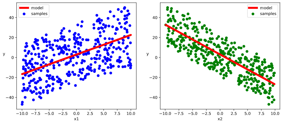
# 结果可视化
%matplotlib inline
%config InlineBackend.figure_format = 'svg'

plt.figure(figsize=(12, 5))
ax1 = plt.subplot(121)
ax1.scatter(X[:, 0], Y[:, 0], c="b", label="samples")
ax1.plot(X[:, 0], w[0]*X[:, 0]+b[0], "-r", linewidth=5.0, label="model")
ax1.legend()
plt.xlabel("x1")
plt.ylabel("y", rotation=0)

ax2 = plt.subplot(122)
ax2.scatter(X[:, 1], Y[:, 0], c='g', label="samples")
ax2.plot(X[:, 1], w[1]*X[:, 1]+b[0], "-r", linewidth=5.0, label="model")
ax2.legend()
plt.xlabel("x2")
plt.ylabel("y", rotation=0)
plt.show()
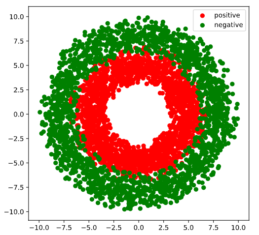
DNN分类模型#
- 准备数据
import numpy as np
import pandas as pd
import matplotlib.pyplot as plt
import tensorflow as tf
%matplotlib inline
%config InlineBackend.figure_format = 'svg'

# 正负样本数量
n_positive, n_negative = 2000, 2000

# 生成正样本,小圆环分布
# 截断正态分布随机数,均值mean,标准差stddev,不过只保留[mean-2stddev,mean+2stddev]范围内的随机数
# 所谓的random_normal服从正太分布的所有随机数,而truncated_normal仅仅只是截取了正太分布某一个范围的数据并不是全部数据
r_p = 5.0 + tf.random.truncated_normal([n_positive, 1], 0.0, 1.0)
theta_p = tf.random.uniform([n_positive, 1], 0.0, 2*np.pi)
Xp = tf.concat([r_p*tf.cos(theta_p), r_p*tf.sin(theta_p)], axis=1)
# 函数目的是创建一个和输入参数(tensor)维度一样,元素都为1的张量
Yp = tf.ones_like(r_p)

# 生成负样本,大圆环分布
r_n = 8.0 + tf.random.truncated_normal([n_negative, 1], 0.0, 1.0)
theta_n = tf.random.uniform([n_negative, 1], 0.0, 2*np.pi)
Xn = tf.concat([r_n*tf.cos(theta_n), r_n*tf.sin(theta_n)], axis=1)
Yn = tf.zeros_like(r_n)

# 汇总样本
X = tf.concat([Xp, Xn], axis=0)
Y = tf.concat([Yp, Yn], axis=0)

# 可视化
plt.figure(figsize=(6, 6))
plt.scatter(Xp[:, 0].numpy(), Xp[:, 1].numpy(), c='r')
plt.scatter(Xn[:, 0].numpy(), Xn[:, 1].numpy(), c='g')
plt.legend(["positive", "negative"])
# 构建数据管道迭代器
def data_iter(features, labels, batch_size=8):
    num_examples = len(features)
    indices = list(range(num_examples))
    np.random.shuffle(indices)  # 样本的读取顺序是随机的
    for i in range(0, num_examples, batch_size):
        indexes = indices[i: min(i+batch_size, num_examples)]
        yield tf.gather(features, indexes), tf.gather(labels, indexes)

# 测试数据管道效果
batch_size = 10
(features, labels) = next(data_iter(X, Y, batch_size))
print(features)
print(labels)

"""
tf.Tensor(
[[ 4.339381   -7.4655576 ]
 [ 7.764667    1.4770296 ]
 [ 2.9533281  -2.7668667 ]
 [ 6.773708   -5.530711  ]
 [-1.0832825   3.794303  ]
 [ 3.4709542   4.1592827 ]
 [ 0.0977866   5.129816  ]
 [ 0.81011575 -6.6931834 ]
 [ 6.4049654  -1.6493047 ]
 [-7.2636695  -4.121036  ]], shape=(10, 2), dtype=float32)
tf.Tensor(
[[0.]
 [0.]
 [1.]
 [0.]
 [1.]
 [1.]
 [1.]
 [1.]
 [1.]
 [0.]], shape=(10, 1), dtype=float32)
"""
- 定义模型
此处范例我们利用tf.Module来组织模型变量,关于tf.Module的比较详细介绍参考第四章最后一节:Autograph和tf.Module
class DNNModel(tf.Module):
    def __init__(self, name=None):
        super(DNNModel, self).__init__(name=name)
        self.w1 = tf.Variable(tf.random.truncated_normal([2, 4]), dtype=tf.float32)
        self.b1 = tf.Variable(tf.zeros([1, 4]), dtype=tf.float32)
        self.w2 = tf.Variable(tf.random.truncated_normal([4, 8]), dtype=tf.float32)
        self.b2 = tf.Variable(tf.zeros([1, 8]), dtype=tf.float32)
        self.w3 = tf.Variable(tf.random.truncated_normal([8, 1]), dtype=tf.float32)
        self.b3 = tf.Variable(tf.zeros([1, 1]), dtype=tf.float32)

    # 正向传播
    # TensorSpec主要由tf使用。函数指定输入签名。tf函数将为不同的输入形状和数据类型创建一个图,
    # 但函数图可能与不同的形状兼容。作为性能优化,您可以选择提供签名,这样就不会创建不必要的图。
    @tf.function(input_signature=[tf.TensorSpec(shape=[None, 2], dtype=tf.float32)])
    def __call__(self, x):
        x = tf.nn.relu(x@self.w1 + self.b1)
        x = tf.nn.relu(x@self.w2 + self.b2)
        y = tf.nn.sigmoid(x@self.w3 + self.b3)
        return y

    # 损失函数(二元交叉熵)
    @tf.function(input_signature=[tf.TensorSpec(shape=[None, 1], dtype=tf.float32), tf.TensorSpec(shape=[None, 1], dtype=tf.float32)])
    def loss_func(self, y_true, y_pred):
        # 将预测值限制在1e-7以上,1-1e-7以下,避免log(0)错误
        eps = 1e-7
        # clip_by_value可以将一个张量中的数值限制在一个范围之内
        y_pred = tf.clip_by_value(y_pred, eps, 1.0-eps)
        bce = - y_true * tf.math.log(y_pred) - (1-y_true) * tf.math.log(1-y_pred)
        return tf.reduce_mean(bce)

    @tf.function(input_signature=[tf.TensorSpec(shape=[None, 1], dtype=tf.float32), tf.TensorSpec(shape=[None, 1], dtype=tf.float32)])
    def metric_func(self, y_true, y_pred):
        y_pred = tf.where(y_pred>0.5, tf.ones_like(y_pred, dtype=tf.float32), tf.zeros_like(y_pred, dtype=tf.float32))
        acc = tf.reduce_mean(1 - tf.abs(y_true - y_pred))
        return acc

model = DNNModel()
# 测试模型结构
batch_size = 10
(features, labels) = next(data_iter(X, Y, batch_size))

predictions = model(features)

loss = model.loss_func(labels, predictions)
metric = model.metric_func(labels, predictions)

tf.print("init loss:", loss)
tf.print("init metric:", metric)

"""
init loss: 10.8162708
init metric: 0.3
"""

print(len(model.trainable_variables))
"""
6
"""
- 训练模型
# 使用autograph机制转换成静态图加速

@tf.function
def train_step(model, features, labels):
    # 正向传播求损失
    with tf.GradientTape() as tape:
        predictions = model(features)
        loss = model.loss_func(labels, predictions)

    # 反向传播求梯度
    grads = tape.gradient(loss, model.trainable_variables)

    # 执行梯度下降
    for p, dloss_dp in zip(model.trainable_variables, grads):
        p.assign(p - 0.001 * dloss_dp)

    # 计算评估指标
    metric = model.metric_func(labels, predictions)
    return loss, metric


def train_model(model, epochs):
    for epoch in tf.range(1, epochs+1):
        for features, labels in data_iter(X, Y, 100):
            loss, metric = train_step(model, features, labels)
        if epoch % 100 == 0:
            printbar()
            tf.print("epoch=", epoch, "loss=", loss, "accuracy=", metric)

train_model(model, epochs=600)

"""
================================================================================21:07:45
epoch= 100 loss= 0.296703756 accuracy= 0.93
================================================================================21:07:48
epoch= 200 loss= 0.277753323 accuracy= 0.9
================================================================================21:07:51
epoch= 300 loss= 0.260072589 accuracy= 0.87
================================================================================21:07:54
epoch= 400 loss= 0.227921337 accuracy= 0.92
================================================================================21:07:57
epoch= 500 loss= 0.191958889 accuracy= 0.91
================================================================================21:08:00
epoch= 600 loss= 0.170489371 accuracy= 0.93
"""
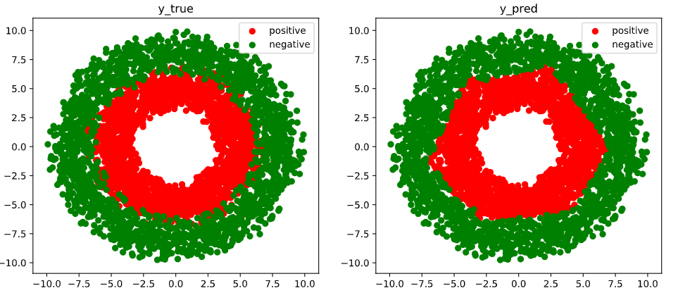
# 结果可视化
fig, (ax1, ax2) = plt.subplots(nrows=1, ncols=2, figsize=(12, 5))
ax1.scatter(Xp[:, 0], Xp[:, 1], c="r")
ax1.scatter(Xn[:, 0], Xn[:, 1], c="g")
ax1.legend(["positive", "negative"])
ax1.set_title("y_true")

# tf.boolean_mask 的作用是 通过布尔值 过滤元素
# tf.squeeze该函数返回一个张量,这个张量是将原始input中所有大小为1的那些维都删掉的结果
Xp_pred = tf.boolean_mask(X, tf.squeeze(model(X) >= 0.5), axis=0)
Xn_pred = tf.boolean_mask(X, tf.squeeze(model(X) < 0.5), axis=0)

ax2.scatter(Xp_pred[:, 0], Xp_pred[:, 1], c="r")
ax2.scatter(Xn_pred[:, 0], Xn_pred[:, 1], c="g")
ax2.legend(["positive", "negative"])
ax2.set_title("y_pred")
作者:lotuslaw
出处:https://www.cnblogs.com/lotuslaw/p/16100538.html
版权:本作品采用「署名-非商业性使用-相同方式共享 4.0 国际」许可协议进行许可。
分类:
TensorFlow


【推荐】国内首个AI IDE,深度理解中文开发场景,立即下载体验Trae
【推荐】编程新体验,更懂你的AI,立即体验豆包MarsCode编程助手
【推荐】抖音旗下AI助手豆包,你的智能百科全书,全免费不限次数
【推荐】轻量又高性能的 SSH 工具 IShell:AI 加持,快人一步
· 阿里最新开源QwQ-32B,效果媲美deepseek-r1满血版,部署成本又又又降低了!
· 开源Multi-agent AI智能体框架aevatar.ai,欢迎大家贡献代码
· Manus重磅发布:全球首款通用AI代理技术深度解析与实战指南
· 被坑几百块钱后,我竟然真的恢复了删除的微信聊天记录!
· 没有Manus邀请码?试试免邀请码的MGX或者开源的OpenManus吧