7-降维
理论部分#
降维的作用#
- 数据降维确实会丢失一些信息,所以,它虽然能够加速训练,但是也会轻微降低系统性能
- 同时它也让流水线更为复杂,维护难度上升,因此,如果训练太慢,你首先应该尝试的还是继续使用原始数据,然后再考虑数据降维
- 不过在某些情况下,降低训练数据的维度可能会滤除掉一些不必要的噪声和细节,从而导致性能更好(但通常来说不会,它只会加速训练)
- 降维对于数据可视化也非常有用,将维度降到两个(或三个),就可以在图形是哪个绘制出高维训练集,通过视觉来检测模式,常常可以获得一些十分重要的洞察,比如聚类
维度的诅咒#
- 高维超立方体中大多数点都非常接近边界
- 高维数据集有很大可能是非常稀疏的:大多数训练实例可能彼此之间相距很远。当然这也意味着新的实例很可能远离任何一个训练实例,导致跟低维度相比,预测更加不可靠,因为它们基于更大的推测。简而言之,训练集的维度越高,过拟合的风险就越大
- 理论上来说,通过增大训练集,使训练实例达到足够的密度,是可以解开维度的诅咒的。然而不幸的是,实践中,要达到给定密度,所需要的训练实例数量随着维度的增加呈指数式上升。
降维的主要方法#
- 减少维度的两种主要方法:投影和流形学习
- 投影
- 在大多数实际问题中,许多特征几乎是恒定不变的,而其他特征则是高度相关的,结果,所有训练实例都位于(或接近于)高维空间的低维子空间内
- 假设高维空间(3D)的所有训练实例都位于一个平面附近(低维子空间,2D),如果我们将每个训练实例垂直投影到该子空间上,则我们将获得新的2D数据集,即将数据集的维度从3D减少到2D
- 投影并不总是降低尺寸的最佳方法,在许多情况下,子空间可能会发生扭曲和转动
- 流形学习
- 一般而言,d维流形是n维空间(其中d<n)的一部分,局部类似于d维超平面。以2D流形为例,2D流形是可以在更高维度的空间中弯曲和扭曲的2D形状
- 许多降维算法通过对训练实例所在的流形进行建模来工作。这称为流形学习,它依赖于流形假说(也称为流形假设),该假设认为大多数现实世界的高维度数据集都接近与低维流形
- 流形假设通常还伴随着另一个隐式假设:如果用流形的低维空间表示,手头的任务(例如分类或回归)将更加简单;但是这种隐含假设并不总是成立。简而言之,在训练模型之前,降低训练集的维度肯定可以加快训练速度,但这并不总是会导致更好或更简单的解决方法,它取决于数据集
PCA#
- 主成分分析(PCA)是迄今为止最流行的降维方法。首先,它识别最靠近数据的超平面,然后将数据投影到其上
- 将训练集投影到低维超平面之前需要选择正确的超平面。选择保留最大差异性的轴看起来比较合理,因为它丢失的信息可能最少。要证明这一选择,还有一种方法,即比较原始数据集与其轴上的投影之间的均方距离,使这个均方距离最小的轴是最合理的选择,这正是PCA背后的简单思想
- 主要成分
- 主成分分析可以在训练集中识别出哪条轴对差异性的贡献度最高。第i个轴称为数据的第i个主要成分(PC),第一个PC是向量c1所在的轴,第二个PC是向量c2所在的轴,前两个PC是对应的轴在平面上正交,第三个PC是与该平面正交的轴
- 利用标准矩阵分解技术(奇异值分解,SVD)可以将训练集矩阵X分解为三个矩阵UΣVT的矩阵乘法,其中V包含定义所有主要成分的单位向量。主成分矩阵:V=(c1, c2, ..., cn)
- PCA假定数据集以原点为中心,如果你自己实现PCA,或者使用其他库,请不要忘记首先将数据居中
- 向下投影到d维度
- 一旦确定了所有主要成分,你就可以将数据集投影到d个主要成分定义的超平面上,从而将数据集的维度降低到d维。选择这个超平面可确保投影将保留尽可能多的差异性
- 可解释方差比
- 另一个有用的信息是每个主成分的可解释方差比,该比例表示沿每个成分的数据集方差的比率
- 例:数据集方差的84.2%位于第一个PC上,而14.6%位于第二个PC上。对于第三个PC,这还不到1.2%,因此可以合理地假设第三个PC携带的信息很少
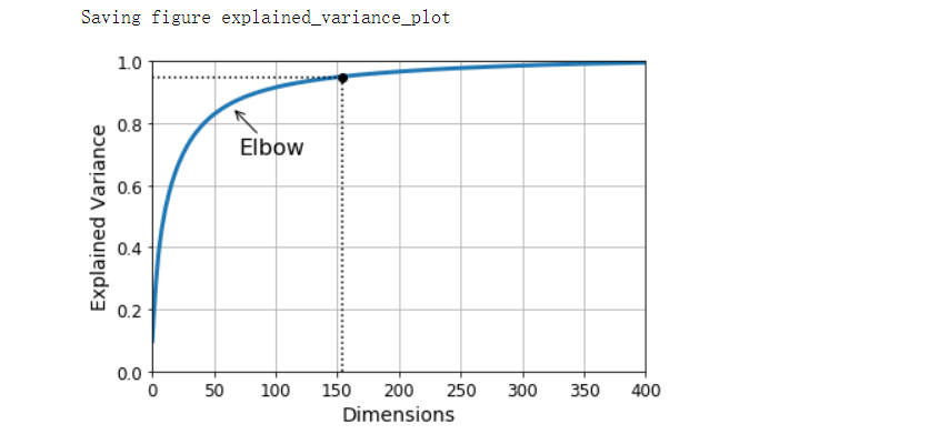
- 选择正确的维度
- 与其任意选择要减小到的维度,不如选择相加足够大的方差部分(例如95%)的维度
- PCA压缩
- 将PCA应用于MNIST数据集,同时保留其95%的方差,你会发现每个实例将具有150多个特征,而不是原始的784个特征。因此尽管保留了大多数方差,但数据集现在不到其原始大小的20%,这是一个合理的压缩率,你可以看到这种维度缩小极大地加速了分类算法
- 通过应用PCA投影的逆变换,还可以将缩减后的数据集解压缩回784维,由于投影会丢失一些信息(5%的方差被丢弃),因此这不会给你原始的距离,但可能会接近原始数据。原始数据与重构数据(压缩后再解压缩)之间的均方距离称为重构误差
- 随机PCA
- Randomized PCA算法可以快速找到前d个主成分的近似值,因此当d远远小于n时,它比完全的SVD快得多
增量PCA#
- PCA实现的一个问题是,它们要求整个训练集都放入内存才能运行算法,而增量PCA(IPCA)算法可以使你把训练集活粉为多个小批量,并一次将一个小批量送入IPCA算法,这对于大型训练集和在线应用PCA很有用
- NumPy的memmap类,使你可以将存储在磁盘上的二进制文件中的大型数组当作完全是内存中一样来操作,该类仅在需要时才将数据加载到内存中
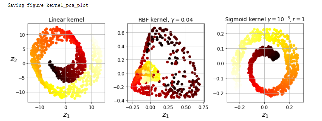
内核PCA#
-
从前述学习中,可以得知内核是一种数学技术,它可以将实例隐式映射到一个高维空间(称为特征空间),从而可以使用支持向量机来进行非线性分类和回归
-
事实证明,可以将相同的技术应用于PCA,从而可以执行复杂的非线性投影来降低维度。这叫作内核PCA(kPCA)。它通常擅长在投影后保留实例的聚类,有时甚至可以展开位于扭曲流形附近的数据集
-
选择内核并调整超参数
- 由于kPCA是一种无监督学习算法,因此没有明显的性能指标可以帮助你选择最好的内核和超参数值。也就是说,降维通常是有监督学习任务(例如分类)的准备步骤,因此你可以使用网格搜索来选择在该任务上能获得最佳性能的内核和超参数
- 另一种完全无监督的方法是选择产生最低重构误差的内核和超参数。如果我们可以对一个给定的实例缩小的空间中反转线性PCA,则重构点将位于特征空间中,而不是原始空间中。由于特征空间是无限维的,因此我们无法计算重构点。幸运的是,有可能在原始空间中找到一个点,该点将映射到重构点附近,这一点称为重建原像。一旦你有了原像,就可以测量其余原始实例的平方距离。然后可以选择内核和超参数,最大限度地减少此重构原像误差。
- 如何执行这个重构?一种解决方案是训练有监督的回归模型,其中将投影实例作为训练集,将原始实例作为目标值
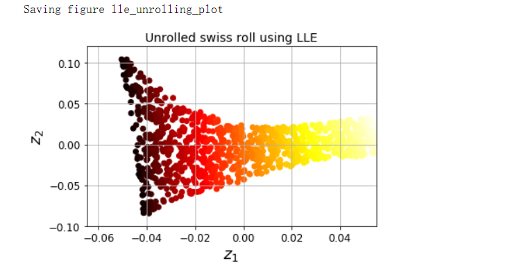
LLE#
- 局部线性嵌入(LLE)是另一种强大的非线性降维(NLDR)技术。它是一种流形学习技术,不像以前的算法那样依赖于投影。简而言之,LLE的工作原理是首先测量每个训练实例如何与其最近的邻居(c.n.)线性相关,然后寻找可以最好地保留这些局部关系的训练集的低维表示。这种方法特别适合展开扭曲的流形,尤其是在没有太多噪声的情况下
其他降维技术#
- 随机投影
- 多维缩放
- Isomap
- t分布随机近邻嵌入
- 线性判别分析(LDA)
代码部分#
引入#
import sys
assert sys.version_info >= (3, 5)
import sklearn
assert sklearn.__version__ >= '0.20'
import numpy as np
import os

np.random.seed(42)

%matplotlib inline
import matplotlib as mpl
import matplotlib.pyplot as plt
mpl.rc('axes', labelsize=14)
mpl.rc('xtick', labelsize=12)
mpl.rc('ytick', labelsize=12)

PROJECT_ROOT_DIR = '.'
CHAPTER_ID = 'dim_reduction'
IMAGES_PATH = os.path.join(PROJECT_ROOT_DIR, 'images', CHAPTER_ID)
os.makedirs(IMAGES_PATH, exist_ok=True)

def save_fig(fig_id, tight_layout=True, fig_extension='png', resolution=300):
    path = os.path.join(IMAGES_PATH, fig_id + '.' + fig_extension)
    print('Saving figure', fig_id)
    if tight_layout:
        plt.tight_layout()
    plt.savefig(path, format=fig_extension, dpi=resolution)
投影法#
np.random.seed(4)
m = 60
w1, w2 = 0.1, 0.3
noise = 0.1

angles = np.random.rand(m) * 3 * np.pi / 2 - 0.5
X = np.empty((m, 3))
X[:, 0] = np.cos(angles) + np.sin(angles)/2 + noise * np.random.randn(m) / 2
X[:, 1] = np.sin(angles) * 0.7 + noise * np.random.randn(m) / 2
X[:, 2] = X[:, 0] * w1 + X[:, 1] * w2 + noise * np.random.randn(m)

# SVD 分解
X_centered = X - X.mean(axis=0)
U, s, Vt = np.linalg.svd(X_centered)
c1 = Vt.T[:, 0]
c2 = Vt.T[:, 1]

m, n = X.shape
S = np.zeros(X_centered.shape)
# 当 np.diag(array) 中
# array是一个1维数组时,结果形成一个以一维数组为对角线元素的矩阵
# array是一个二维矩阵时,结果输出矩阵的对角线元素
S[:n, :n] = np.diag(s)

# numpy的allclose方法,比较两个array是不是每一元素都相等,默认在1e-05的误差范围内
np.allclose(X_centered, U.dot(S).dot(Vt))  # True

W2 = Vt.T[:, :2]
X2D = X_centered.dot(W2)

X2D_using_svd = X2D

# sklearn
from sklearn.decomposition import PCA

pca = PCA(n_components=2)
X2D = pca.fit_transform(X)

np.allclose(X2D, -X2D_using_svd)  # True

# 解压缩
X3D_inv = pca.inverse_transform(X2D)

np.allclose(X3D_inv, X)  # False

# 重构原像误差
np.mean(np.sum(np.square(X3D_inv - X), axis=1))  # 0.010170337792848549

# SVD 解压缩
X3D_inv_using_svd = X2D_using_svd.dot(Vt[:2, :])

np.allclose(X3D_inv_using_svd, X3D_inv - pca.mean_)  # True

# 主成分
pca.components_  # array([[-0.93636116, -0.29854881, -0.18465208], [ 0.34027485, -0.90119108, -0.2684542 ]])

# SVD 主成分
Vt[:2]  # array([[ 0.93636116,  0.29854881,  0.18465208], [-0.34027485,  0.90119108,  0.2684542 ]])

# 可解释方差比
pca.explained_variance_ratio_  # array([0.84248607, 0.14631839])

1 - sum(pca.explained_variance_ratio_)  # 0.011195535570688975

# SVD 可解释方差比
np.square(s) / np.square(s).sum()  # array([0.84248607, 0.14631839, 0.01119554])
投影#
from matplotlib.patches import FancyArrowPatch
from mpl_toolkits.mplot3d import proj3d

class Arrow3D(FancyArrowPatch):
    def __init__(self, xs, ys, zs, *args, **kwargs):
        FancyArrowPatch.__init__(self, (0, 0), (0, 0), *args, **kwargs)
        self._verts3d = xs, ys, zs

    def draw(self, renderer):
        xs3d, ys3d, zs3d = self._verts3d
        xs, ys, zs = proj3d.proj_transform(xs3d, ys3d, zs3d, renderer.M)
        self.set_positions((xs[0], ys[0]), (xs[1], ys[1]))
        FancyArrowPatch.draw(self, renderer)

axes = [-1.8, 1.8, -1.3, 1.3, -1.0, 1.0]

x1s = np.linspace(axes[0], axes[1], 10)
x2s = np.linspace(axes[2], axes[3], 10)
x1, x2 = np.meshgrid(x1s, x2s)

C = pca.components_
R = C.T.dot(C)
z = (R[0, 2] * x1 + R[1, 2] * x2) / (1 - R[2, 2])
from mpl_toolkits.mplot3d import Axes3D

fig = plt.figure(figsize=(6, 3.8))
ax = fig.add_subplot(111, projection='3d')

X3D_above = X[X[:, 2] > X3D_inv[:, 2]]
X3D_below = X[X[:, 2] <= X3D_inv[:, 2]]

ax.plot(X3D_below[:, 0], X3D_below[:, 1], X3D_below[:, 2], 'bo', alpha=0.5)
ax.plot_surface(x1, x2, z, alpha=0.2, color='k')

np.linalg.norm(C, axis=0)

ax.add_artist(Arrow3D([0, C[0, 0]], [0, C[0, 1]], [0, C[0, 2]], mutation_scale=15, lw=1, arrowstyle='-|>', color='k'))
ax.add_artist(Arrow3D([0, C[1, 0]], [0, C[1, 1]], [0, C[1, 2]], mutation_scale=15, lw=1, arrowstyle='-|>', color='k'))
ax.plot([0], [0], [0], 'k.')

for i in range(m):
    if X[i, 2] > X3D_inv[i, 2]:
        ax.plot([X[i][0], X3D_inv[i][0]], [X[i][1], X3D_inv[i][1]], [X[i][2], X3D_inv[i][2]], 'k-')
    else:
        ax.plot([X[i][0], X3D_inv[i][0]], [X[i][1], X3D_inv[i][1]], [X[i][2], X3D_inv[i][2]], 'k-', color='#505050')

ax.plot(X3D_inv[:, 0], X3D_inv[:, 1], X3D_inv[:, 2], 'k+')
ax.plot(X3D_inv[:, 0], X3D_inv[:, 1], X3D_inv[:, 2], 'k.')
ax.plot(X3D_above[:, 0], X3D_above[:, 1], X3D_above[:, 2], 'bo')
ax.set_xlabel('$x_1$', fontsize=18, labelpad=10)
ax.set_ylabel('$x_2$', fontsize=18, labelpad=10)
ax.set_zlabel('$x_3$', fontsize=18, labelpad=10)
ax.set_xlim(axes[:2])
ax.set_ylim(axes[2:4])
ax.set_zlim(axes[4:6])
save_fig('dataset_3d_plot')
plt.show()
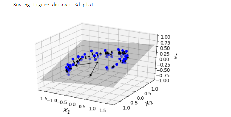
fig = plt.figure()
ax = fig.add_subplot(111, aspect='equal')
ax.plot(X2D[:, 0], X2D[:, 1], 'k+')
ax.plot(X2D[:, 0], X2D[:, 1], 'k.')
ax.plot([0], [0], 'ko')
ax.arrow(0, 0, 0, 1, head_width=0.05, length_includes_head=True, head_length=0.1, fc='k', ec='k')
ax.arrow(0, 0, 1, 0, head_width=0.05, length_includes_head=True, head_length=0.1, fc='k', ec='k')
ax.set_xlabel('$z_1$', fontsize=18)
ax.set_ylabel('$z_2$', fontsize=18, rotation=0)
ax.axis([-1.5, 1.3, -1.2, 1.2])
ax.grid(True)
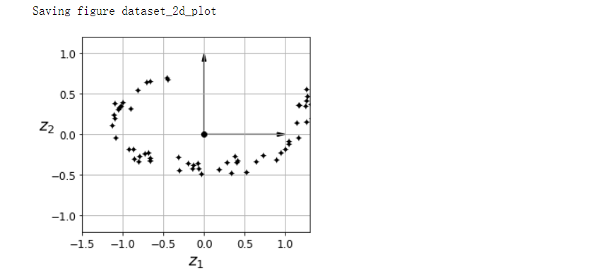
save_fig('dataset_2d_plot')
流形学习#
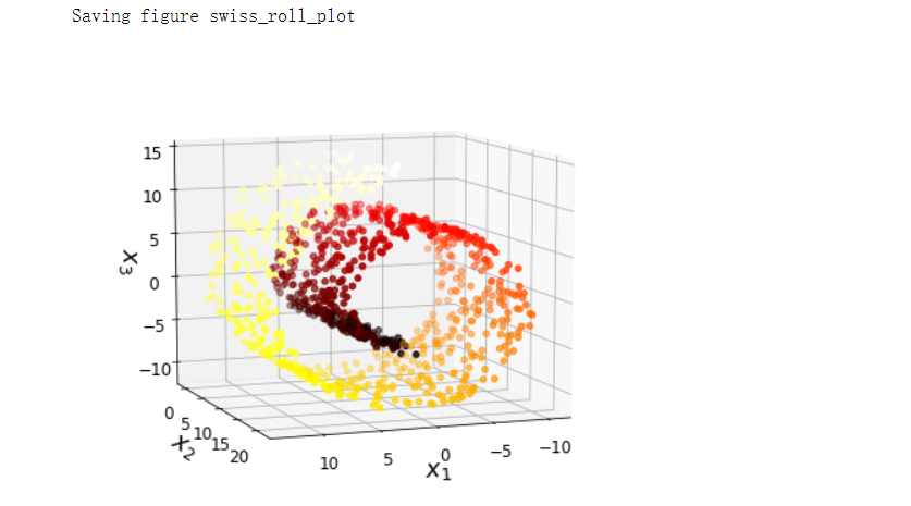
# 瑞士卷数据集
from sklearn.datasets import make_swiss_roll

X, t = make_swiss_roll(n_samples=1000, noise=0.2, random_state=42)

axes = [-11.5, 14, -2, 23, -12, 15]
fig = plt.figure(figsize=(6, 5))
ax = fig.add_subplot(111, projection='3d')
ax.scatter(X[:, 0], X[:, 1], X[:, 2], c=t, cmap=plt.cm.hot)
ax.view_init(10, 70)
ax.set_xlabel('$x_1$', fontsize=18)
ax.set_ylabel('$x_2$', fontsize=18)
ax.set_zlabel('$x_3$', fontsize=18)
ax.set_xlim(axes[0:2])
ax.set_ylim(axes[2:4])
ax.set_zlim(axes[4:6])
save_fig('swiss_roll_plot')
plt.show()
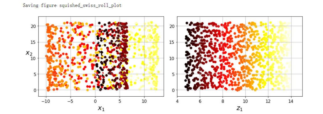
# 左右两张子图的y是同样的,区别在于x
plt.figure(figsize=(11, 4))
plt.subplot(121)
plt.scatter(X[:, 0], X[:, 1], c=t, cmap=plt.cm.hot)
plt.axis(axes[:4])
plt.xlabel('$x_1$', fontsize=18)
plt.ylabel('$x_2$', fontsize=18, rotation=0)
plt.grid(True)

plt.subplot(122)
plt.scatter(t, X[:, 1], c=t, cmap=plt.cm.hot)
plt.axis([4, 15, axes[2], axes[3]])
plt.xlabel('$z_1$', fontsize=18)
plt.grid(True)

save_fig('squished_swiss_roll_plot')
plt.show()
from matplotlib import gridspec

axes = [-11.5, 14, -2, 23, -12, 15]

x2s = np.linspace(axes[2], axes[3], 10)
x3s = np.linspace(axes[4], axes[5], 10)
x2, x3 = np.meshgrid(x2s, x3s)
fig = plt.figure(figsize=(6, 5))
ax = plt.subplot(111, projection='3d')
positive_class = X[:, 0] > 5
X_pos = X[positive_class]
X_neg = X[~positive_class]
ax.view_init(10, 70)
ax.plot(X_neg[:, 0], X_neg[:, 1], X_neg[:, 2], 'y^')
ax.plot_wireframe(5, x2, x3, alpha=0.5)
ax.plot(X_pos[:, 0], X_pos[:, 1], X_pos[:, 2], 'gs')
ax.set_xlabel('$x_1$', fontsize=18)
ax.set_ylabel('$x_2$', fontsize=18)
ax.set_zlabel('$x_3$', fontsize=18)
ax.set_xlim(axes[0:2])
ax.set_ylim(axes[2:4])
ax.set_zlim(axes[4:6])
save_fig('manifold_decision_boundary_plot1')
plt.show()

fig = plt.figure(figsize=(5, 4))
ax = plt.subplot(111)

plt.plot(t[positive_class], X[positive_class, 1], 'gs')
plt.plot(t[~positive_class], X[~positive_class, 1], 'y^')
plt.axis([4, 15, axes[2], axes[3]])
plt.xlabel('$z_1$', fontsize=18)
plt.ylabel('$z_2$', fontsize=18, rotation=0)
plt.grid(True)

save_fig('manifold_decision_boundary_plot2')
plt.show()
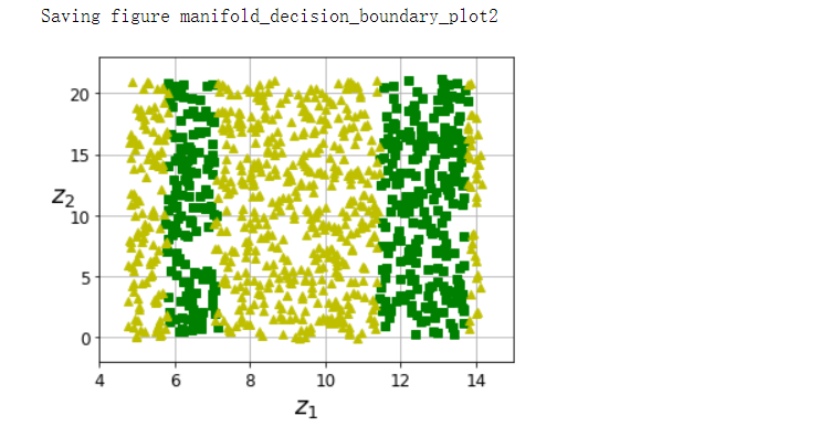
fig = plt.figure(figsize=(6, 5))
ax = plt.subplot(111, projection='3d')

positive_class = 2 * (t[:] - 4) > X[:, 1]
X_pos = X[positive_class]
X_neg = X[~positive_class]
# 转换视角进行观察
ax.view_init(10, 70)
ax.plot(X_neg[:, 0], X_neg[:, 1], X_neg[:, 2], 'y^')
ax.plot(X_pos[:, 0], X_pos[:, 1], X_pos[:, 2], 'gs')
ax.set_xlabel('$x_1$', fontsize=18)
ax.set_ylabel('$x_2$', fontsize=18)
ax.set_zlabel('$x_3$', fontsize=18)
ax.set_xlim(axes[0:2])
ax.set_ylim(axes[2:4])
ax.set_zlim(axes[4:6])
save_fig('manifold_decision_boundary_plot3')
plt.show()
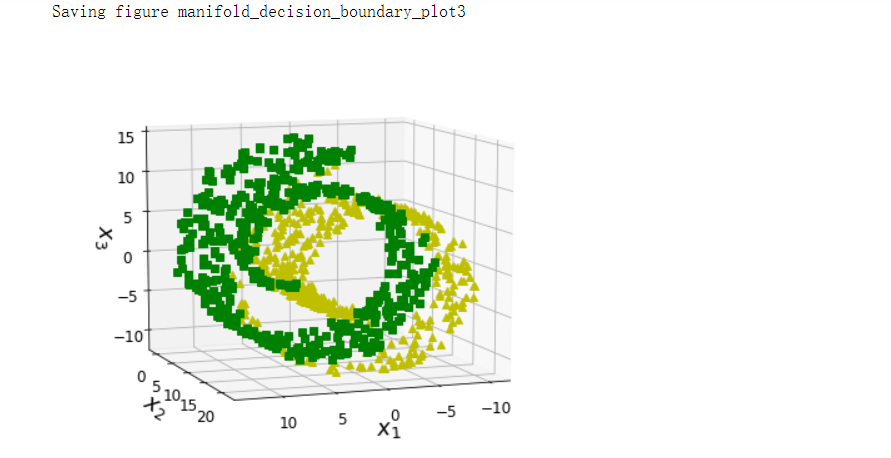
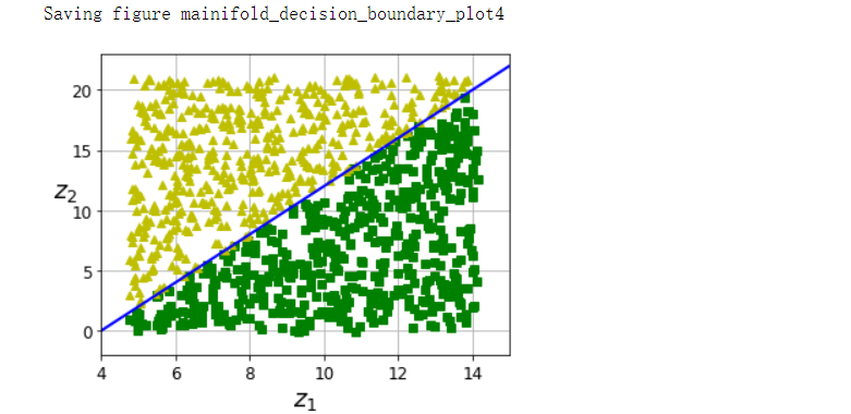
fig = plt.figure(figsize=(5, 4))
ax = plt.subplot(111)
plt.plot(t[positive_class], X[positive_class, 1], 'gs')
plt.plot(t[~positive_class], X[~positive_class, 1], 'y^')
plt.plot([4, 15], [0, 22], 'b-', linewidth=2)
plt.axis([4, 15, axes[2], axes[3]])
plt.xlabel('$z_1$', fontsize=18)
plt.ylabel('$z_2$', fontsize=18, rotation=0)
plt.grid(True)
save_fig('mainifold_decision_boundary_plot4')
plt.show()
PCA#
angle = np.pi / 5
stretch = 5
m = 200

np.random.seed(3)
X = np.random.randn(m, 2) / 10
X = X.dot(np.array([[stretch, 0], [0, 1]]))  # stretch
X = X.dot([[np.cos(angle), np.sin(angle)], [-np.sin(angle), np.cos(angle)]])  # rotation

u1 = np.array([np.cos(angle), np.sin(angle)])
u2 = np.array([np.cos(angle - 2 * np.pi/6), np.sin(angle - 2 * np.pi/6)])
u3 = np.array([np.cos(angle - np.pi/2), np.sin(angle - np.pi/2)])

X_proj1 = X.dot(u1.reshape(-1, 1))
X_proj2 = X.dot(u2.reshape(-1, 1))
X_proj3 = X.dot(u3.reshape(-1, 1))

plt.figure(figsize=(8, 4))
# 画子图,三行两列
plt.subplot2grid((3, 2), (0, 0), rowspan=3)
plt.plot([-1.4, 1.4], [-1.4*u1[1]/u1[0], 1.4*u1[1]/u1[0]], 'k-', linewidth=1)
plt.plot([-1.4, 1.4], [-1.4*u2[1]/u2[0], 1.4*u2[1]/u2[0]], 'k--', linewidth=1)
plt.plot([-1.4, 1.4], [-1.4*u3[1]/u3[0], 1.4*u3[1]/u3[0]], 'k:', linewidth=2)
plt.plot(X[:, 0], X[:, 1], 'bo', alpha=0.5)
plt.axis([-1.4, 1.4, -1.4, 1.4])
plt.arrow(0, 0, u1[0], u1[1], head_width=0.1, linewidth=5, length_includes_head=True, head_length=0.1, fc='k', ec='k')
plt.arrow(0, 0, u3[0], u3[1], head_width=0.1, linewidth=5, length_includes_head=True, head_length=0.1, fc='k', ec='k')
plt.text(u1[0] + 0.1, u1[1] - 0.05, r'$\mathbf{c_1}$', fontsize=22)
plt.text(u3[0] + 0.1, u3[1], r'$\mathbf{c_2}$', fontsize=22)
plt.xlabel('$x_1$', fontsize=18)
plt.ylabel('$x_2$', fontsize=18, rotation=0)
plt.grid(True)

plt.subplot2grid((3, 2), (0, 1))
plt.plot([-2, 2], [0, 0], 'k-', linewidth=1)
plt.plot(X_proj1[:, 0], np.zeros(m), 'bo', alpha=0.3)
plt.gca().get_yaxis().set_ticks([])
plt.gca().get_xaxis().set_ticklabels([])
plt.axis([-2, 2, -1, 1])
plt.grid(True)

plt.subplot2grid((3, 2), (1, 1))
plt.plot([-2, 2], [0, 0], 'k--', linewidth=1)
plt.plot(X_proj2[:, 0], np.zeros(m), 'bo', alpha=0.3)
plt.gca().get_yaxis().set_ticks([])
plt.gca().get_xaxis().set_ticklabels([])
plt.axis([-2, 2, -1, 1])
plt.grid(True)

plt.subplot2grid((3, 2), (2, 1))
plt.plot([-2, 2], [0, 0], 'k:', linewidth=2)
plt.plot(X_proj3[:, 0], np.zeros(m), 'bo', alpha=0.3)
plt.gca().get_yaxis().set_ticks([])
plt.axis([-2, 2, -1, 1])
plt.xlabel('$z_1$', fontsize=18)

save_fig('pca_best_projection_plot')
plt.show()

选择正确的维度#
from sklearn.datasets import fetch_openml

mnist = fetch_openml('mnist_784', version=1, as_frame=False)
mnist.target = mnist.target.astype(np.uint8)

from sklearn.model_selection import train_test_split

X = mnist['data']
y = mnist['target']

X_train, X_test, y_train, y_test = train_test_split(X, y)

pca = PCA()
pca.fit(X_train)
cumsum = np.cumsum(pca.explained_variance_ratio_)
d = np.argmax(cumsum >= 0.95) + 1

d  # 154
plt.figure(figsize=(6, 4))
plt.plot(cumsum, linewidth=3)
plt.axis([0, 400, 0, 1])
plt.xlabel('Dimensions')
plt.ylabel('Explained Variance')
plt.plot([d, d], [0, 0.95], 'k:')
plt.plot([0, d], [0.95, 0.95], 'k:')
plt.plot(d, 0.95, 'ko')
plt.annotate('Elbow', xy=(65, 0.85), xytext=(70, 0.7), arrowprops=dict(arrowstyle='->'), fontsize=16)
plt.grid(True)
save_fig('explained_variance_plot')
plt.show()
pca = PCA(n_components=0.95)
X_reduced = pca.fit_transform(X_train)
pca.n_components_ # 154
np.sum(pca.explained_variance_ratio_) # 0.9504334914295707
pca = PCA(n_components=154)
X_reduced = pca.fit_transform(X_train)
X_recovered = pca.inverse_transform(X_reduced)
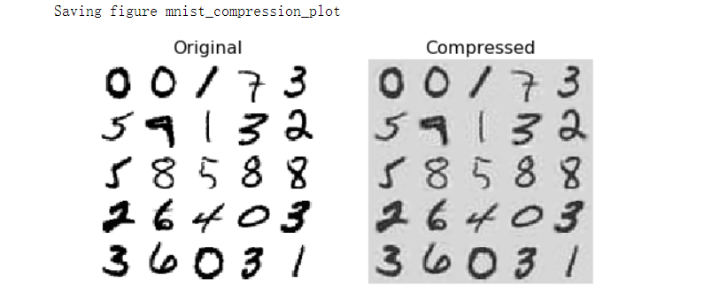
def plot_digits(instances, images_per_row=5, **options):
size = 28
images_per_row = min(len(instances), images_per_row)
images = [instance.reshape(size, size) for instance in instances]
n_rows = (len(instances) - 1) // images_per_row + 1
row_images = []
n_empty = n_rows * images_per_row - len(instances)
images.append(np.zeros((size, size * n_empty)))
for row in range(n_rows):
rimages = images[row * images_per_row : (row + 1) * images_per_row]
row_images.append(np.concatenate(rimages, axis=1))
image = np.concatenate(row_images, axis=0)
plt.imshow(image, cmap=mpl.cm.binary, **options)
plt.axis('off')
plt.figure(figsize=(7, 4))
plt.subplot(121)
plot_digits(X_train[::2100])
plt.title('Original', fontsize=16)
plt.subplot(122)
plot_digits(X_recovered[::2100])
plt.title('Compressed', fontsize=16)
save_fig('mnist_compression_plot')
X_reduced_pca = X_reduced
增量PCA#
from sklearn.decomposition import IncrementalPCA

n_batches = 100
inc_pca = IncrementalPCA(n_components=154)
for X_batch in np.array_split(X_train, n_batches):
    print('.', end='')
    inc_pca.partial_fit(X_batch)
X_reduced = inc_pca.transform(X_train)

X_recovered_inc_pca = inc_pca.inverse_transform(X_reduced)

plt.figure(figsize=(7, 4))
plt.subplot(121)
plot_digits(X_train[::2100])
plt.subplot(122)
plot_digits(X_recovered_inc_pca[::2100])
plt.tight_layout()
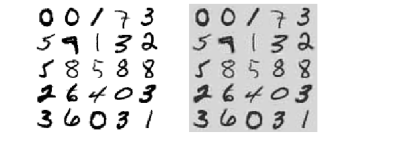
X_reduced_inc_pca = X_reduced

# 每个feature的平均值。在pca算法的第一步,需要对feature归一化,此时的平均值保留在这里
np.allclose(pca.mean_, inc_pca.mean_)  # True

np.allclose(X_reduced_pca, X_reduced_inc_pca)  # False
使用memmap#
filename = r'my_mnist.data'
m, n = X_train.shape

X_mm = np.memmap(filename, dtype='float32', mode='write', shape=(m, n))
X_mm[:] = X_train

del X_mm

X_mm = np.memmap(filename, dtype='float32', mode='readonly', shape=(m, n))
batch_size = m // n_batches
inc_pca = IncrementalPCA(n_components=154, batch_size=batch_size)
inc_pca.fit(X_mm)
随机PCA#
rnd_pca = PCA(n_components=154, svd_solver='randomized', random_state=42)
X_reduced = rnd_pca.fit_transform(X_train)
时间复杂度#
import time

for n_components in (2, 10, 154):
    print('n_components = ', n_components)
    regular_pca = PCA(n_components=n_components, svd_solver='full')
    inc_pca = IncrementalPCA(n_components=n_components, batch_size=500)
    rnd_pca = PCA(n_components=n_components, random_state=42, svd_solver='randomized')

    for name, pca in (('PCA', regular_pca), ('Inc PCA', inc_pca), ('Rnd PCA', rnd_pca)):
        t1 = time.time()
        pca.fit(X_train)
        t2 = time.time()
        print('{}: {:.1f} seconds'.format(name, t2 - t1))
'''
n_components =  2
PCA: 6.0 seconds
Inc PCA: 18.5 seconds
Rnd PCA: 2.4 seconds
n_components =  10
PCA: 7.6 seconds
Inc PCA: 22.7 seconds
Rnd PCA: 2.9 seconds
n_components =  154
PCA: 7.0 seconds
Inc PCA: 29.7 seconds
Rnd PCA: 5.1 seconds
'''
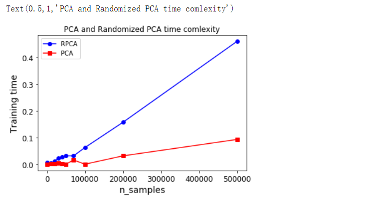
times_rpca = []
times_pca = []
sizes = [1000, 10000, 20000, 30000, 40000, 50000, 70000, 100000, 200000, 500000]
for n_samples in sizes:
    X = np.random.randn(n_samples, 5)
    pca = PCA(n_components=2, svd_solver='randomized', random_state=42)
    t1 = time.time()
    pca.fit(X)
    t2 = time.time()
    times_rpca.append(t2 - t1)
    pca = PCA(n_components=2, svd_solver='full')
    t1 = time.time()
    pca.fit(X)
    t2 = time.time()
    times_pca.append(t2 - t1)

plt.plot(sizes, times_rpca, 'b-o', label='RPCA')
plt.plot(sizes, times_pca, 'r-s', label='PCA')
plt.xlabel('n_samples')
plt.ylabel('Training time')
plt.legend(loc='upper left')
plt.title('PCA and Randomized PCA time comlexity')
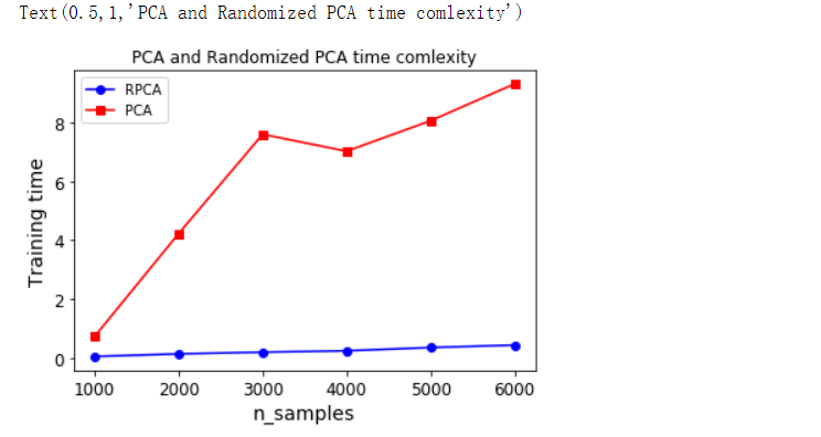
times_rpca = []
times_pca = []
sizes = [1000, 2000, 3000, 4000, 5000, 6000]
for n_features in sizes:
    X = np.random.randn(2000, n_features)
    pca = PCA(n_components=2, svd_solver='randomized', random_state=42)
    t1 = time.time()
    pca.fit(X)
    t2 = time.time()
    times_rpca.append(t2 - t1)
    pca = PCA(n_components=2, svd_solver='full')
    t1 = time.time()
    pca.fit(X)
    t2 = time.time()
    times_pca.append(t2 - t1)

plt.plot(sizes, times_rpca, 'b-o', label='RPCA')
plt.plot(sizes, times_pca, 'r-s', label='PCA')
plt.xlabel('n_samples')
plt.ylabel('Training time')
plt.legend(loc='upper left')
plt.title('PCA and Randomized PCA time comlexity')
核PCA#
X, t = make_swiss_roll(n_samples=1000, noise=0.2, random_state=42)

from sklearn.decomposition import KernelPCA

rbf_pca = KernelPCA(n_components=2, kernel='rbf', gamma=0.04)
X_reduced = rbf_pca.fit_transform(X)

from sklearn.decomposition import KernelPCA

lin_pca = KernelPCA(n_components=2, kernel='linear', fit_inverse_transform=True)
rbf_pca = KernelPCA(n_components=2, kernel='rbf', gamma=0.0433, fit_inverse_transform=True)
sig_pca = KernelPCA(n_components=2, kernel='sigmoid', gamma=0.001, coef0=1, fit_inverse_transform=True)

y = t > 6.9

plt.figure(figsize=(11, 4))
for subplot, pca, title in ((131, lin_pca, 'Linear kernel'), (132, rbf_pca, 'RBF kernel, $\gamma=0.04$'), (133, sig_pca, 'Sigmoid kernel $\gamma=10^{-3}, r=1$')):
    X_reduced = pca.fit_transform(X)
    if subplot == 132:
        X_reduced_rbf = X_reduced

    plt.subplot(subplot)
    plt.title(title, fontsize=14)
    plt.scatter(X_reduced[:, 0], X_reduced[:, 1], c=t, cmap=plt.cm.hot)
    plt.xlabel('$z_1$', fontsize=18)
    if subplot == 131:
        plt.ylabel('$z_2$', fontsize=18, rotation=0)
    plt.grid(True)

save_fig('kernel_pca_plot')
plt.show()
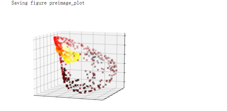
plt.figure(figsize=(6, 5))
X_inverse = rbf_pca.inverse_transform(X_reduced_rbf)
ax = plt.subplot(111, projection='3d')
ax.view_init(10, -70)
ax.scatter(X_inverse[:, 0], X_inverse[:, 1], X_inverse[:, 2], c=t, cmap=plt.cm.hot, marker='x')
ax.set_xlabel('')
ax.set_ylabel('')
ax.set_zlabel('')
ax.set_xticklabels([])
ax.set_yticklabels([])
ax.set_zticklabels([])

save_fig('preimage_plot', tight_layout=False)
plt.show()
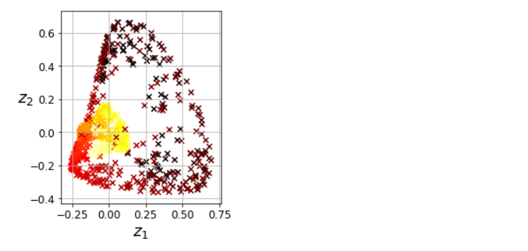
X_reduced = rbf_pca.fit_transform(X)
plt.figure(figsize=(11, 4))
plt.subplot(132)
plt.scatter(X_reduced[:, 0], X_reduced[:, 1], c=t, cmap=plt.cm.hot, marker='x')
plt.xlabel('$z_1$', fontsize=18)
plt.ylabel('$z_2$', fontsize=18, rotation=0)
plt.grid(True)
网格搜索调优#
from sklearn.model_selection import GridSearchCV
from sklearn.linear_model import LogisticRegression
from sklearn.pipeline import Pipeline

reg = Pipeline([
    ('kpca', KernelPCA(n_components=2)),
    ('log_reg', LogisticRegression(solver='lbfgs'))
])
param_grid = [{
    'kpca__gamma': np.linspace(0.03, 0.05, 10),
    'kpca__kernel': ['rbf', 'sigmoid']
}]
grid_search = GridSearchCV(reg, param_grid, cv=3)
grid_search.fit(X, y)

print(grid_search.best_params_)  # {'kpca__gamma': 0.043333333333333335, 'kpca__kernel': 'rbf'}

rbf_pca = KernelPCA(n_components=2, kernel='rbf', gamma=0.0433, fit_inverse_transform=True)
X_reduced = rbf_pca.fit_transform(X)
X_preimage = rbf_pca.inverse_transform(X_reduced)

from sklearn.metrics import mean_squared_error

mean_squared_error(X, X_preimage)  # 32.78630879576614
LLE#
X, t = make_swiss_roll(n_samples=1000, noise=0.2, random_state=41)

from sklearn.manifold import LocallyLinearEmbedding

lle = LocallyLinearEmbedding(n_components=2, n_neighbors=10, random_state=42)
X_reduced = lle.fit_transform(X)

plt.title('Unrolled swiss roll using LLE', fontsize=14)
plt.scatter(X_reduced[:, 0], X_reduced[:, 1], c=t, cmap=plt.cm.hot)
plt.xlabel('$z_1$', fontsize=18)
plt.ylabel('$z_2$', fontsize=18)
plt.axis([-0.065, 0.055, -0.1, 0.12])
plt.grid(True)

save_fig('lle_unrolling_plot')
plt.show()
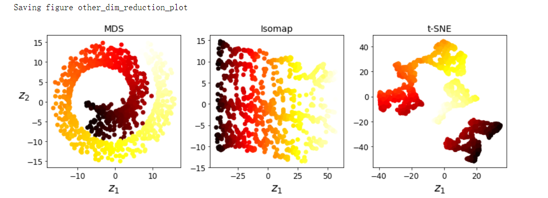
多维缩放(MDS), Isomap and t分布随机近邻嵌入(t-SNE)#
from sklearn.manifold import MDS

mds = MDS(n_components=2, random_state=42)
X_reduced_mds = mds.fit_transform(X)

from sklearn.manifold import Isomap

isomap = Isomap(n_components=2)
X_reduced_isomap = isomap.fit_transform(X)

from sklearn.manifold import TSNE

tsne = TSNE(n_components=2, random_state=42)
X_reduced_tsne = tsne.fit_transform(X)

from sklearn.discriminant_analysis import LinearDiscriminantAnalysis

lda = LinearDiscriminantAnalysis(n_components=2)
X_mnist = mnist['data']
y_mnist = mnist['target']
lda.fit(X_mnist, y_mnist)
X_reduced_lda = lda.transform(X_mnist)

titles = ['MDS', 'Isomap', 't-SNE']
plt.figure(figsize=(11, 4))
for subplot, title, X_reduced in zip((131, 132, 133), titles, (X_reduced_mds, X_reduced_isomap, X_reduced_tsne)):
    plt.subplot(subplot)
    plt.title(title, fontsize=14)
    plt.scatter(X_reduced[:, 0], X_reduced[:, 1], c=t, cmap=plt.cm.hot)
    plt.xlabel('$z_1$', fontsize=18)
    if subplot == 131:
        plt.ylabel('$z_2$', fontsize=18, rotation=0)
    plt.grid=True

save_fig('other_dim_reduction_plot')
plt.show()
作者:lotuslaw
出处:https://www.cnblogs.com/lotuslaw/p/15547617.html
版权:本作品采用「署名-非商业性使用-相同方式共享 4.0 国际」许可协议进行许可。


【推荐】国内首个AI IDE,深度理解中文开发场景,立即下载体验Trae
【推荐】编程新体验,更懂你的AI,立即体验豆包MarsCode编程助手
【推荐】抖音旗下AI助手豆包,你的智能百科全书,全免费不限次数
【推荐】轻量又高性能的 SSH 工具 IShell:AI 加持,快人一步
· 开发者必知的日志记录最佳实践
· SQL Server 2025 AI相关能力初探
· Linux系列:如何用 C#调用 C方法造成内存泄露
· AI与.NET技术实操系列(二):开始使用ML.NET
· 记一次.NET内存居高不下排查解决与启示
· 阿里最新开源QwQ-32B,效果媲美deepseek-r1满血版,部署成本又又又降低了!
· 开源Multi-agent AI智能体框架aevatar.ai,欢迎大家贡献代码
· Manus重磅发布:全球首款通用AI代理技术深度解析与实战指南
· 被坑几百块钱后,我竟然真的恢复了删除的微信聊天记录!
· 没有Manus邀请码?试试免邀请码的MGX或者开源的OpenManus吧
2020-11-13 7-时间序列分析基础-有待深入研究
2020-11-13 6-KKT条件
2020-11-13 5-正则化
2020-11-13 4-梯度下降法
2020-11-13 3-线性回归的正则化:Ridge回归及Lasso回归
2020-11-13 2-线性回归及其推广
2020-11-13 1-KNN