6-集成学习和随机森林
理论部分#
随机森林定义#
- 训练一组决策树分类器,每一棵树都基于训练集不同的随机子集进行训练。做出预测时,你只需要获得所有树各自的预测,然后给出得票最多的类别作为预测结果,这样一组决策树的集成被称为随机森林
投票分类器#
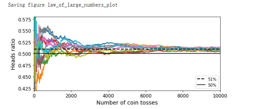
- 要创建出一个更好的分类器,最简单的办法就是聚合每个分类器的预测,然后将得票最多的结果作为预测类别,这种大多数投票分类器被称为硬投票分类器
- 如果所有分类器都能够估算出类别的概率,那么你可以将概率在所有单个分类器上平均,然后让概率最高的类别作为预测,这被称为软投票法,通常来说,它比硬投票法的表现更优,因为它给予那些高度自信的投票更高的权重
- 当预测器尽可能相互独立时,集成方法的效果最优
bagging和pasting#
- 获取不同种分类器的方法之一是使用不同的训练算法,还有另一种方法是每个预测器使用的算法相同,但是在不同的训练集随机子集上进行训练。采样时如果将样本放回,这种方法叫作bagging(bootstrap aggregating的缩写,也叫自举汇聚法)。采样时样本不放回,这种方法叫作pasting
- 一旦预测器训练完成,集成就可以通过简单地聚合所有预测器的预测来对新实例做出预测。聚合函数通常是统计法(即最多数的预测与硬投票分类器一样)用于分类,或是平均法用于回归。每个预测器单独的偏差都高于在原始训练集上训练的偏差,但是通过聚合,同时降低了偏差和方差,总体来说,最终结果是,与直接在原始训练集上训练的单个预测器相比,集成的偏差相近,但是方差更低。
- 由于自举法给每个预测器的训练子集引入了更高的多样性,所以最后bagging比pasting的偏差略高,但这也意味着预测器之间的关联度更低,所以集成的方差降低。总之,bagging生成的模型通常更好,这也就是为什么它更受欢迎
包外估计#
- 对于给定的预测器,使用bagging,有些实例可能会被采样多次,而有些实例则可能根本不被采样。这意味着对每个预测器来说,平均只对63%的训练实例进行采样,剩余37%未被采样的训练实例称为包外(oob)实例。由于预测器在训练过程中从未看到oob实例,因此可以在这些实例上进行评估,而无须单独的验证集。你可以通过平均每个预测器的oob评估来评估整体
随机补丁和随机子空间#
- 采用特征采样后,每个预测器将用输入特征的随机子集进行训练,这对于处理高维输入(例如图像)特别有用,对训练实例和特征都进行抽样,这称为随机补丁方法
- 保留所有训练实例但对特征进行抽样,这被称为随机子空间法
- 对特征抽样给预测器带来更大的多样性,所以以略高一点的偏差换取了更低的方差
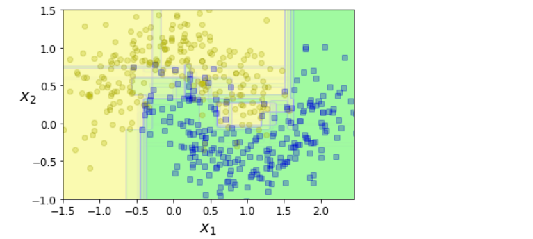
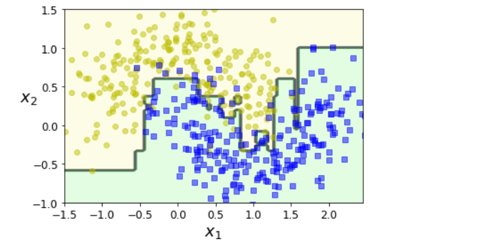
随机森林#
- 随机森林在树的生长上引入了更多的随机性,分裂节点时不再是搜索最好的特征,而是在一个随机生成的特征子集里搜索最好的特征。这导致决策树具有更大的多样性,用更高的偏差换取更低的方差,总之,还是产生了一个整体性能更优的模型
- 极端随机树
- 在随机森林里单棵树的生长过程中,每个节点在分裂时仅考虑到了一个随机子集所包含的特征,如果我们对每个特征使用随机阈值,而不是搜索得出最佳的阈值,则可能让决策树生长得更加随机。这种极端随机的决策树组成的森林称为极端随机树集成(或简称Extra-Trees)。它也是以更高的偏差换取了更低的方差。极端随机树训练起来比常规随机森林要快得多,因为在每个节点上找到每个特征的最佳阈值是决策树生长中最耗时的任务之一
- 与随机森林的优劣对比需要进行实际比较
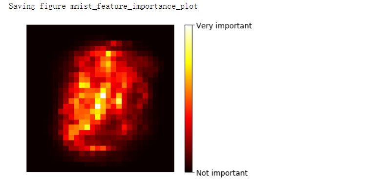
- 特征重要性
- 随机森林的另一个好特性是它们使测量每个特征的相对重要性变得容易。通过查看使用该特征的树节点平均(在森林中的所有树上)减少不纯度的程度来衡量该特征的重要性。更准确的说,它是一个加权平均值,其中每个节点的权重等于与其关联的训练样本的数量
提升法#
- 提升法(boosting,最初被称为假设提升)是指可以将几个弱学习器结合成一个强学习器的任意集成方法。大多数提升法的总体思路是循环训练预测器,每一次都对其前序做出一些改正。可用的提升法有很多,但目前最流行的方法是AdaBoost和梯度提升
- AdaBoost
- 新预测器对其前序进行纠正的方法之一就是更多地关注前序欠拟合的训练实例,从而使新的预测器不断地越来越专注于难缠的问题,这就是AdaBoost使用的技术。当训练AdaBoost分类器时,该算法首先训练一个基础分类器(例如决策树),并使用它对训练集进行预测。然后,该算法会增加分类错误的训练实例的相对权重。然后,它使用更新后的权重训练第二个分类器,并再次对训练集进行预测,更新实例权重,以此类推
- AdaBoost这种依序循环的学习技术跟梯度下降有一些异曲同工之处,差别只在于不再是调整单个预测器的参数使成本函数最小化,而是不断在集成中加入预测器,使模型越来越好
- 一旦全部预测器训练完成,集成整体做出预测时就跟bagging或pasting方法一样,除非预测器有不同的权重,因为它们总的准确率是基于加权后的训练集
- 这种依序学习技术有一个重要的缺陷就是无法并行,因为每个预测器只能在前一个预测器训练完成并评估之后才能开始训练。因此在扩展方面,它的表现不如bagging和pasting方法
- AdaBoost的多分类版本,叫作SAMME(基于多类指数损失函数的逐步添加模型)。当只有两类时,SAMME即等同于AdaBoost。此外,如果预测器可以估算概率,可以使用SAMME的变体,称为SAMME.R,它依赖的是类概率而不是类预测,通常表现更好
梯度提升#
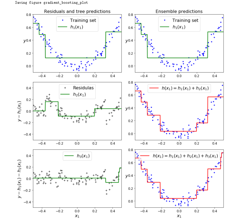
- 梯度提升也是逐步在集成中添加预测器,每一个都对其前序做出改正。不同之处在于,它不是像AdaBoost那样,在每个迭代中调整实例权重,而是让新的预测器针对前一个预测器的残差进行拟合。
- GBDT
- 来源:GBDT详解 - 白开水加糖 - 博客园 (cnblogs.com)
- GBDT(Gradient Boosting Decision Tree)又叫MART(Multiple Additive Regression Tree),是一种迭代的决策树算法,该算法由多棵决策树组成,所有树的结论累加起来做最终答案。它在被提出之初就和SVM一起被认为是泛化能力(generalization)较强的算法。
- DT:回归树Regression Decision Tree
- 提起决策树,绝大部分人首先想到的就是分类决策树,但如果一开始就把GBDT中的树想成分类树,那就是一条歪路走到黑。决策树分为两大类,回归树和分类树。前者用于预测实数值,如温度;后者用于分类标签值,如晴天/阴天。这里要强调的是,前者的结果加减是有意义的,后者则无意义。GBDT的核心在于累加所有树的结果作为最终结果,就像对年龄的累加,所以GBDT中的树都是回归树,而不是分类树,这点对理解GBDT相当重要
- 对于分类CART树,试图最小化的成本函数是分裂后左右子树的加权基尼系数最小;而对于回归CART树,其试图最小化的成本函数是分裂后,左右子树的加权MSE最小,分裂完成后,每个节点的预测值等于这个节点的所有取值的均值
- GB:梯度迭代Gradient Boosting
- Boosting,迭代,即通过迭代多棵树来共同决策。GBDT的核心就在于,每一棵树学的是之前所有树结论和的残差,这个残差就是一个加预测值后能得到真实值的累加量
- GBDT工作流程
- 既然用一棵树就可以拟合出100%精度的模型,为什么要用多棵树迭代?答案就是过拟合。过拟合是指为了让训练集精度更高,学到了很多“仅在训练集上成立的规律”,导致换一个数据集后,当前的规律就不适用了。Boosting的最大好处在于,每一步的残差计算其实变相地增大了分错instance的权重,而已经分队的instance则都趋向于0。这样后面的树就能越来越专注于那些前面被分错的instance。就像我们做互联网,总是先解决60%用户的需求,再解决35%用户的需求,最后才关注那5%的人的需求,这样就能逐渐把产品做好,因为不同类型用户需求可能完全不同,需要分别独立分析。如果反过来做,或者刚上来就一定要做到尽善尽美,往往都会竹篮打水一场空
- 到目前为止,我们的确没有用到求导的Gradient,因为用残差作为全局最优的绝对方向,并不需要Gradient求解
- GBDT也可以在使用残差的同时引入Bootstrap re-sampling,GBDT多数实现版本中也增加了这个选项,但是否一定有用,则有不同看法。re-sampling一个缺点是它的随机性,即同样的数据集合训练两遍结果是不一样的,也就是模型不可稳定复现,这对评估是很大挑战,比如很那说一个模型变好是因为你选用了更好的feature,还是由于这次sample的随机因素。这种方法也是用更高的偏差换取了更低方差,同时在相当大的程度上加速了训练过程,这种技术被称为随机梯度提升
- Shrinkage
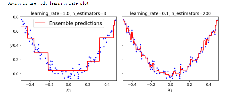
- Shrinkage(缩减)的思想认为,每次走一小步逐步逼近结果的效果,要比每次迈一大步很快逼近结果的方式更容易避免过拟合。即它不完全信任每一颗残差树,它认为每棵树只学到了真理的一小部分,累加的时候只累加一小部分,通过多学几棵树弥补不足。
- Shrinkage仍然以残差作为学习目标,但对于残差学习出来的结果,只累加一小部分逐步逼近目标,step一般都比较小,导致各个树的残差是渐变的而不是陡变的。直觉上这也很好理解,不像直接用残差一步修复误差,而是只修复一点点,其实就是把大步切成了很多小步。本质上,Shrinkage为每棵树设置了一个weight,累加时要乘以这个weight,但和Gradient并没有关系。
- 适用范围
- 几乎可用于所有的线性/非线性回归问题;也可以用于分类问题(设置阈值,大于阈值为正例,反之为反例)


-
XGBoost
-
流行的Python库XGBoost(该库代表Extreme Gradient Boosting)中提供了梯度提升的优化实现,该软件包最初是由陈天齐作为分布式(深度)机器学习社区(DMLC)的一部分开发的,其开发目标是极快、可扩展和可移植。
-
目标函数
-
-
分裂节点的方法
- 枚举所有树结构的贪心法
- 不断地枚举不同树的结构,然后利用打分函数来寻找出一个最优结构的树,接着加入到模型中,不断重复这样的操作。这个寻找的过程使用的就是贪心算法。选择一个feature分裂,计算loss function最小值,然后再选一个feature分裂,又得到以loss function最小值,枚举完找到一个效果最好的,进行分裂
-
XGBoost与GBDT有什么不同
- GBDT是机器学习算法,XGBoost是该算法的工程实现
- 在使用CART作为基分类器时,XGBoost显示地加入了正则项来控制模型的复杂度,有利于防止过拟合,从而提高模型的泛化能力
- GBDT在模型训练时只使用了损失函数的一阶导数信息,XGBoost对损失函数进行二阶泰勒展开,可以同时使用一阶和二阶导数
- 传统的GBDT采用CART作为基分类器,XGBoost支持多种类型的基分类器,比如线性分类器
- 传统的GBDT在每轮迭代时使用全部的数据,XGBoost则采用了与随机森林相似的策略,支持对数据进行采样
- 传统的GBDT没有设计对缺失值进行处理,XGBoost能够自动学习出缺失值的处理策略
-
为什么XGBoost要用二阶泰勒展开,优势在哪里?
- XGBoost使用了一阶和二阶偏导,二阶导数有利于梯度下降的更快更准。使用泰勒展开取得函数做自变量的二阶导数形式,可以在不选定损失函数具体形式的情况下,仅仅依靠输入数据的值就可以进行叶子分裂优化计算,本质上就是把损失函数的选取和模型算法优化/参数选择分开了。这种去耦合增加了XGBoost的适用性,使得它按需选取损失函数,可用于分类,也可用于回归
-
堆叠法#
- 堆叠法又称层叠泛化法,它基于一个简单的想法:与其使用一些简单的函数(比如硬投票)来聚合集成中所有预测器的预测,我们为什么不训练一个模型来执行这个聚合呢?例如在新实例上执行回归任务的这样一个集成。底部的n个预测器分别预测了不同的值,然后最终的预测器(称为混合器或元学习器)将这些预测作为输入,进行最终预测
- 训练混合器的常用方法是使用留存集
- 首先将训练集分为两个子集,第一个子集用来训练第一层的预测器
- 然后用第一层的预测器在第二个(留存)子集上进行预测。因为预测器在训练时从未见过这些实例,所以可以确保预测是“干净的”。那么现在对于留存集中的每个实例都有了三个预测值。我们可以使用这些预测值作为输入特征,创建一个新的训练集(新的训练集有三个维度),并保留目标值。在这个新的训练集上训练混合器,让它学习根据第一层的预测来预测目标值
代码部分#
引入#
import sys
assert sys.version_info >= (3, 5)

import sklearn
assert sklearn.__version__ >= '0.20'

import numpy as np
import os

np.random.seed(42)

%matplotlib inline

import matplotlib as mpl
import matplotlib.pyplot as plt
mpl.rc('axes', labelsize=14)
mpl.rc('xtick', labelsize=12)
mpl.rc('ytick', labelsize=12)

PROJECT_ROOT_DIR = '.'
CHAPTER_ID = 'ensembles'
IMAGES_PATH = os.path.join(PROJECT_ROOT_DIR, 'images', CHAPTER_ID)
os.makedirs(IMAGES_PATH, exist_ok=True)

def save_fig(fig_id, tight_layout=True, fig_extension='png', resolution=300):
    path = os.path.join(IMAGES_PATH, fig_id + '.' + fig_extension)
    print("Saving figure", fig_id)
    if tight_layout:
        plt.tight_layout()
    plt.savefig(path, format=fig_extension, dpi=resolution)
硬投票#
heads_proba = 0.51
coin_tosses = (np.random.rand(10000, 10) < heads_proba).astype(np.int32)
# 求数组的所有元素的累计和,可通过参数axis指定求某个轴向的统计值。
# 模拟1万次掷骰子,掷1次-10000次的概率,cumsum实现累加
cumulative_heads_ratio = np.cumsum(coin_tosses, axis=0) / np.arange(1, 10001).reshape(-1, 1)

plt.figure(figsize=(8, 3.5))
plt.plot(cumulative_heads_ratio)
plt.plot([0, 10000], [0.51, 0.51], 'k--', linewidth=2, label='51%')
plt.plot([0, 10000], [0.5, 0.5], 'k-', label='50%')
plt.xlabel('Number of coin tosses')
plt.ylabel('Heads ratio')
plt.legend(loc='lower right')
plt.axis([0, 10000, 0.42, 0.58])
save_fig('law_of_large_numbers_plot')
plt.show()
from sklearn.model_selection import train_test_split
from sklearn.datasets import make_moons

X, y = make_moons(n_samples=500, noise=0.30, random_state=42)
X_train, X_test, y_train, y_test = train_test_split(X, y, random_state=42)

from sklearn.ensemble import RandomForestClassifier
from sklearn.ensemble import VotingClassifier
from sklearn.linear_model import LogisticRegression
from sklearn.svm import SVC

log_clf = LogisticRegression(solver='lbfgs', random_state=42)
rnd_clf = RandomForestClassifier(n_estimators=100, random_state=42)
svm_clf = SVC(gamma='scale', random_state=42)

voting_clf = VotingClassifier(
    estimators=[('lr', log_clf), ('rf', rnd_clf), ('svc', svm_clf)],
    voting='hard'
)

voting_clf.fit(X_train, y_train)

from sklearn.metrics import accuracy_score

for clf in (log_clf, rnd_clf, svm_clf, voting_clf):
    clf.fit(X_train, y_train)
    y_pred = clf.predict(X_test)
    print(clf.__class__.__name__, accuracy_score(y_test, y_pred))
'''
LogisticRegression 0.864
RandomForestClassifier 0.896
SVC 0.896
VotingClassifier 0.912
'''
软投票#
log_clf = LogisticRegression(solver='lbfgs', random_state=42)
rnd_clf = RandomForestClassifier(n_estimators=100, random_state=42)
svm_clf = SVC(gamma='scale', probability=True, random_state=42)

voting_clf = VotingClassifier(
    estimators=[('lr', log_clf), ('rf', rnd_clf), ('svc', svm_clf)],
    voting='soft'
)
voting_clf.fit(X_train, y_train)

from sklearn.metrics import accuracy_score

for clf in (log_clf, rnd_clf, svm_clf, voting_clf):
    clf.fit(X_train, y_train)
    y_pred = clf.predict(X_test)
    print(clf.__class__.__name__, accuracy_score(y_test, y_pred))
'''
LogisticRegression 0.864
RandomForestClassifier 0.896
SVC 0.896
VotingClassifier 0.92
'''
Bagging#
from sklearn.ensemble import BaggingClassifier
from sklearn.tree import DecisionTreeClassifier

bag_clf = BaggingClassifier(
    DecisionTreeClassifier(),
    n_estimators=500,
    max_samples=100,
    bootstrap=True,
    random_state=42
)
bag_clf.fit(X_train, y_train)
y_pred = bag_clf.predict(X_test)

from sklearn.metrics import accuracy_score

print(accuracy_score(y_test, y_pred))  # 0.904

tree_clf = DecisionTreeClassifier(random_state=42)
tree_clf.fit(X_train, y_train)
y_pred_tree = tree_clf.predict(X_test)
print(accuracy_score(y_test, y_pred_tree))  # 0.856
from matplotlib.colors import ListedColormap

def plot_decision_boundary(clf, X, y, axes=[-1.5, 2.45, -1, 1.5], alpha=0.5, contour=True):
    x1s = np.linspace(axes[0], axes[1], 100)
    x2s = np.linspace(axes[2], axes[3], 100)
    x1, x2 = np.meshgrid(x1s, x2s)
    X_new = np.c_[x1.ravel(), x2.ravel()]
    y_pred = clf.predict(X_new).reshape(x1.shape)
    custom_cmap = ListedColormap(['#fafab0', '#9898ff', '#a0faa0'])
    plt.contourf(x1, x2, y_pred, alpha=0.3, cmap=custom_cmap)
    if contour:
        custom_cmap2 = ListedColormap(['#7d7d58', '#4c4c7f', '#507d50'])
        plt.contour(x1, x2, y_pred, cmap=custom_cmap2, alpha=0.8)
    plt.plot(X[:, 0][y==0], X[:, 1][y==0], 'yo', alpha=alpha)
    plt.plot(X[:, 0][y==1], X[:, 1][y==1], 'bs', alpha=alpha)
    plt.axis(axes)
    plt.xlabel(r'$x_1$', fontsize=18)
    plt.ylabel(r'$x_2$', fontsize=18, rotation=0)

fix, axes = plt.subplots(ncols=2, figsize=(10, 4), sharey=True)
plt.sca(axes[0])
plot_decision_boundary(tree_clf, X, y)
plt.title('Decision Tree', fontsize=14)
plt.sca(axes[1])
plot_decision_boundary(bag_clf, X, y)
plt.title('Decision Trees with Bagging', fontsize=14)
plt.ylabel("")
save_fig('decision_tree_without_and_with_bagging_plot')
plt.show()

随机森林#
bag_clf = BaggingClassifier(
    DecisionTreeClassifier(max_features='sqrt', max_leaf_nodes=16),
    n_estimators=500,
    random_state=42
)

bag_clf.fit(X_train, y_train)
y_pred = bag_clf.predict(X_test)

from sklearn.ensemble import RandomForestClassifier

rnd_clf = RandomForestClassifier(n_estimators=500, max_leaf_nodes=16, random_state=42)
rnd_clf.fit(X_train, y_train)

y_pred_rf = rnd_clf.predict(X_test)

np.sum(y_pred == y_pred_rf) / len(y_pred)  # 1.0
集成学习算法输出特征重要性#
from sklearn.datasets import load_iris

iris = load_iris()
rnd_clf = RandomForestClassifier(n_estimators=500, random_state=42)
rnd_clf.fit(iris['data'], iris['target'])
for name, score in zip(iris['feature_names'], rnd_clf.feature_importances_):
    print(name, score)
'''
sepal length (cm) 0.11249225099876375
sepal width (cm) 0.02311928828251033
petal length (cm) 0.4410304643639577
petal width (cm) 0.4233579963547682
rnd_clf.feature_importances_
'''
rnd_clf.feature_importances_  # array([0.11249225, 0.02311929, 0.44103046, 0.423358  ])
plt.figure(figsize=(6, 4))

for i in range(15):
    tree_clf = DecisionTreeClassifier(max_leaf_nodes=16, random_state=42+i)
    indices_with_replacement = np.random.randint(0, len(X_train), len(X_train))
    tree_clf.fit(X[indices_with_replacement], y[indices_with_replacement])
    plot_decision_boundary(tree_clf, X, y, axes=[-1.5, 2.45, -1, 1.5], alpha=0.02, contour=False)

plt.show()
包外估计#
bag_clf = BaggingClassifier(
    DecisionTreeClassifier(),
    n_estimators=500,
    bootstrap=True,
    oob_score=True,
    random_state=40
)
bag_clf.fit(X_train, y_train)
bag_clf.oob_score_  # 0.8986666666666666

# 决策函数返回的是每个实例的类别概率
bag_clf.oob_decision_function_

from sklearn.metrics import accuracy_score

y_pred = bag_clf.predict(X_test)
accuracy_score(y_test, y_pred)  # 0.912
特征重要性#
from sklearn.datasets import fetch_openml

mnist = fetch_openml('mnist_784', version=1, as_frame=False)
mnist.target = mnist.target.astype(np.uint8)

rnd_clf = RandomForestClassifier(n_estimators=100, random_state=42)
rnd_clf.fit(mnist['data'], mnist['target'])

def plot_digit(data):
    image = data.reshape(28, 28)
    plt.imshow(image, cmap=mpl.cm.hot, interpolation='nearest')
    plt.axis('off')

plot_digit(rnd_clf.feature_importances_)
cbar = plt.colorbar(ticks=[rnd_clf.feature_importances_.min(), rnd_clf.feature_importances_.max()])
cbar.ax.set_yticklabels(['Not important', 'Very important'])
save_fig('mnist_feature_importance_plot')
plt.show()
AdaBoost#
from sklearn.ensemble import AdaBoostClassifier

ada_clf = AdaBoostClassifier(
    DecisionTreeClassifier(max_depth=1),
    n_estimators=200,
    algorithm='SAMME.R',
    learning_rate=0.5,
    random_state=42
)
ada_clf.fit(X_train, y_train)

plot_decision_boundary(ada_clf, X, y)
m = len(X_train)
fix, axes = plt.subplots(ncols=2, figsize=(10, 4), sharey=True)
for subplot, learning_rate in ((0, 1), (1, 0.5)):
    # 初始化1/m
    sample_weights = np.ones(m) / m
    plt.sca(axes[subplot])
    for i in range(5):
        svm_clf = SVC(kernel='rbf', C=0.2, gamma=0.6, random_state=42)
        svm_clf.fit(X_train, y_train, sample_weight=sample_weights * m)
        y_pred = svm_clf.predict(X_train)
        # 预测器的加权误差率
        r = sample_weights[y_pred != y_train].sum() / sample_weights.sum()
        # 预测器权重
        alpha = learning_rate * np.log((1 - r) / r)
        # 权重更新
        sample_weights[y_pred != y_train] *= np.exp(alpha)
        sample_weights /= sample_weights.sum()

        plot_decision_boundary(svm_clf, X, y, alpha=0.2)
        plt.title('learning_rate={}'.format(learning_rate), fontsize=16)
    if subplot == 0:
        plt.text(-0.75, -0.95, '1', fontsize=14)
        plt.text(-1.05, -0.95, '2', fontsize=14)
        plt.text(1.0, -0.95, '3', fontsize=14)
        plt.text(-1.45, -0.5, '4', fontsize=14)
        plt.text(1.36, -0.95, '5', fontsize=14)
    else:
        plt.ylabel('')

save_fig('boosting_plot')
plt.show()

梯度提升#
np.random.seed(42)
X = np.random.rand(100, 1) - 0.5
y = 3 * X[:, 0]**2 + 0.05 * np.random.randn(100)

from sklearn.tree import DecisionTreeRegressor

tree_reg1 = DecisionTreeRegressor(max_depth=2, random_state=42)
tree_reg1.fit(X, y)

y2 = y - tree_reg1.predict(X)
tree_reg2 = DecisionTreeRegressor(max_depth=2, random_state=42)
tree_reg2.fit(X, y2)

y3 = y2 - tree_reg2.predict(X)
tree_reg3 = DecisionTreeRegressor(max_depth=2, random_state=42)
tree_reg3.fit(X, y3)

X_new = np.array([[0.8]])
y_pred = sum(tree.predict(X_new) for tree in (tree_reg1, tree_reg2, tree_reg3))
y_pred  # array([0.75026781])
def plot_predicitions(regressors, X, y, axes, label=None, style='r-', data_style='b.', data_label=None):
    x1 = np.linspace(axes[0], axes[1], 500)
    y_pred = sum(regressor.predict(x1.reshape(-1, 1)) for regressor in regressors)
    plt.plot(X[:, 0], y, data_style, label=data_label)
    plt.plot(x1, y_pred, style, linewidth=2, label=label)
    if label or data_label:
        plt.legend(loc='upper center', fontsize=16)
    plt.axis(axes)

plt.figure(figsize=(11, 11))

plt.subplot(321)
plot_predicitions([tree_reg1], X, y, axes=[-0.5, 0.5, -0.1, 0.8], label='$h_1(x_1)$', style='g-', data_label='Training set')
plt.ylabel('$y$', fontsize=16, rotation=0)
plt.title('Residuals and tree predictions', fontsize=16)

plt.subplot(322)
plot_predicitions([tree_reg1], X, y, axes=[-0.5, 0.5, -0.1, 0.8], label='$h_1(x_1)$', style='g-', data_label='Training set')
plt.ylabel('$y$', fontsize=16, rotation=0)
plt.title('Ensemble predictions', fontsize=16)

plt.subplot(323)
plot_predicitions([tree_reg2], X, y2, axes=[-0.5, 0.5, -0.5, 0.5], label='$h_2(x_1)$', style='g-', data_style='k+', data_label='Residulas')
plt.ylabel('$y - h_1(x_1)$', fontsize=16)

plt.subplot(324)
plot_predicitions([tree_reg1, tree_reg2], X, y, axes=[-0.5, 0.5, -0.1, 0.8], label='$h(x_1) = h_1(x_1) + h_2(x_1)$')
plt.ylabel('$y$', fontsize=16, rotation=0)

plt.subplot(325)
plot_predicitions([tree_reg3], X, y3, axes=[-0.5, 0.5, -0.5, 0.5], label='$h_3(x_1)$', style='g-', data_style='k+')
plt.ylabel('$y - h_1(x_1) -h_2(x_1)$', fontsize=16)
plt.xlabel('$x_1$', fontsize=16)

plt.subplot(326)
plot_predicitions([tree_reg1, tree_reg2, tree_reg3], X, y, axes=[-0.5, 0.5, -0.1, 0.8], label='$h(x_1) = h_1(x_1) + h_2(x_1) + h_3(x_1)$')
plt.xlabel('$x_1$', fontsize=16)
plt.ylabel('$y$', fontsize=16, rotation=0)

save_fig('gradient_boosting_plot')
plt.show()
from sklearn.ensemble import GradientBoostingRegressor

gbdt = GradientBoostingRegressor(max_depth=2, n_estimators=3, learning_rate=1.0, random_state=42)
gbdt.fit(X, y)

gbdt_slow = GradientBoostingRegressor(max_depth=2, n_estimators=200, learning_rate=0.1, random_state=42)
gbdt_slow.fit(X, y)

fix, axes = plt.subplots(ncols=2, figsize=(10, 4), sharey=True)

plt.sca(axes[0])
plot_predicitions([gbdt], X, y, axes=[-0.5, 0.5, -0.1, 0.8], label='Ensemble predictions')
plt.title('learning_rate={}, n_estimators={}'.format(gbdt.learning_rate, gbdt.n_estimators), fontsize=14)
plt.xlabel('$x_1$', fontsize=16)
plt.ylabel('$y$', fontsize=16, rotation=0)

plt.sca(axes[1])
plot_predicitions([gbdt_slow], X, y, axes=[-0.5, 0.5, -0.1, 0.8])
plt.title('learning_rate={}, n_estimators={}'.format(gbdt_slow.learning_rate, gbdt_slow.n_estimators), fontsize=14)
plt.xlabel('$x_1$', fontsize=16)

save_fig('gbdt_learning_rate_plot')
plt.show()
GBDT提前停止法#
import numpy as np
from sklearn.model_selection import train_test_split
from sklearn.metrics import mean_squared_error
X_train, X_val, y_train, y_val = train_test_split(X, y, random_state=49)
gbdt = GradientBoostingRegressor(max_depth=2, n_estimators=120, random_state=42)
gbdt.fit(X_train, y_train)
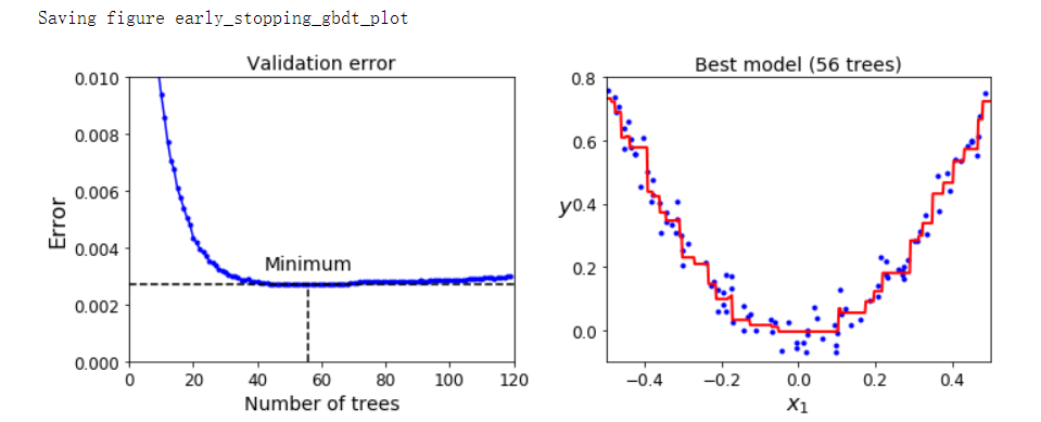
errors = [mean_squared_error(y_val, y_pred) for y_pred in gbdt.staged_predict(X_val)]
bst_n_estimators = np.argmin(errors) + 1
gbdt_best = GradientBoostingRegressor(max_depth=2, n_estimators=bst_n_estimators, random_state=42)
gbdt_best.fit(X_train, y_train)
min_error = np.min(errors)
plt.figure(figsize=(10, 4))
plt.subplot(121)
plt.plot(errors, 'b.-')
plt.plot([bst_n_estimators, bst_n_estimators], [0, min_error], 'k--')
plt.plot([0, 120], [min_error, min_error], 'k--')
plt.text(bst_n_estimators, min_error*1.2, 'Minimum', ha='center', fontsize=14)
plt.axis([0, 120, 0, 0.01])
plt.xlabel('Number of trees')
plt.ylabel('Error', fontsize=16)
plt.title('Validation error', fontsize=14)
plt.subplot(122)
plot_predicitions([gbdt_best], X, y, axes=[-0.5, 0.5, -0.1, 0.8])
plt.title('Best model (%d trees)' % bst_n_estimators, fontsize=14)
plt.ylabel('$y$', fontsize=16, rotation=0)
plt.xlabel('$x_1$', fontsize=16)
save_fig('early_stopping_gbdt_plot')
plt.show()
gbdt = GradientBoostingRegressor(max_depth=2, warm_start=True, random_state=42)

min_val_error = float('inf')
error_going_up = 0
for n_estimators in range(1, 120):
    gbdt.n_estimators = n_estimators
    gbdt.fit(X_train, y_train)
    y_pred = gbdt.predict(X_val)
    val_error = mean_squared_error(y_val, y_pred)
    if val_error < min_val_error:
        min_val_error = val_error
        error_going_up = 0
    else:
        error_going_up += 1
        if error_going_up == 5:
            break

print(gbdt.n_estimators)  # 61

print('Minimum validation MSE:', min_val_error)  # Minimum validation MSE: 0.002712853325235463
XGBoost#
try:
    import xgboost
except ImportError as ex:
    print('Error: the xgboost library is not intalled')
    xgboost = None

if xgboost is not None:
    xgb_reg = xgboost.XGBRegressor(random_state=42)
    xgb_reg.fit(X_train, y_train)
    y_pred = xgb_reg.predict(X_val)
    val_error = mean_squared_error(y_val, y_pred)
    print('Validation MSE:', val_error)  # Validation MSE: 0.004000408205406276
if xgboost is not None:
    xgb_reg.fit(X_train, y_train, eval_set=[(X_val, y_val)], early_stopping_rounds=2)
    y_pred = xgb_reg.predict(X_val)
    val_error = mean_squared_error(y_val, y_pred)
    print('Validation MSE:', val_error)
'''
[0]	validation_0-rmse:0.22834
[1]	validation_0-rmse:0.16224
[2]	validation_0-rmse:0.11843
[3]	validation_0-rmse:0.08760
[4]	validation_0-rmse:0.06848
[5]	validation_0-rmse:0.05709
[6]	validation_0-rmse:0.05297
[7]	validation_0-rmse:0.05129
[8]	validation_0-rmse:0.05155
[9]	validation_0-rmse:0.05211
Validation MSE: 0.002630868681577655
'''

%timeit xgboost.XGBRegressor().fit(X_train, y_train)  # 88.1 ms ± 3.58 ms per loop (mean ± std. dev. of 7 runs, 10 loops each)

%timeit GradientBoostingRegressor().fit(X_train, y_train)  # 19.8 ms ± 484 µs per loop (mean ± std. dev. of 7 runs, 100 loops each)
Stacking Ensemble#
X_train_val, X_test, y_train_val, y_test = train_test_split(mnist.data, mnist.target, test_size=10000, random_state=42)
X_train, X_val, y_train, y_val = train_test_split(X_train_val, y_train_val, test_size=10000, random_state=42)

from sklearn.ensemble import RandomForestClassifier, ExtraTreesClassifier
from sklearn.svm import  LinearSVC
from sklearn.neural_network import MLPClassifier
from sklearn.utils import shuffle

random_forest_clf = RandomForestClassifier(n_estimators=100, random_state=42)
extra_trees_clf = ExtraTreesClassifier(n_estimators=100, random_state=42)
svm_clf = LinearSVC(max_iter=100, tol=20, random_state=42)
mlp_clf = MLPClassifier(random_state=42)

estimators = [random_forest_clf, extra_trees_clf, svm_clf, mlp_clf]
for estimator in estimators:
    print('Training the', estimator)
    estimator.fit(X_train, y_train)

X_val_predictions = np.empty((len(X_val), len(estimators)), dtype=np.float32)
for index, estimator in enumerate(estimators):
    X_val_predictions[:, index] = estimator.predict(X_val)

X_val_predictions
'''
array([[5., 5., 5., 5.],
       [8., 8., 8., 8.],
       [2., 2., 3., 2.],
       ...,
       [7., 7., 7., 7.],
       [6., 6., 6., 6.],
       [7., 7., 7., 7.]], dtype=float32)
'''
rnd_forest_blender = RandomForestClassifier(n_estimators=200, oob_score=True, random_state=42)
rnd_forest_blender.fit(X_val_predictions, y_val)
rnd_forest_blender.oob_score_  # 0.9683
作者:lotuslaw
出处:https://www.cnblogs.com/lotuslaw/p/15543843.html
版权:本作品采用「署名-非商业性使用-相同方式共享 4.0 国际」许可协议进行许可。


【推荐】国内首个AI IDE,深度理解中文开发场景,立即下载体验Trae
【推荐】编程新体验,更懂你的AI,立即体验豆包MarsCode编程助手
【推荐】抖音旗下AI助手豆包,你的智能百科全书,全免费不限次数
【推荐】轻量又高性能的 SSH 工具 IShell:AI 加持,快人一步
· 开发者必知的日志记录最佳实践
· SQL Server 2025 AI相关能力初探
· Linux系列:如何用 C#调用 C方法造成内存泄露
· AI与.NET技术实操系列(二):开始使用ML.NET
· 记一次.NET内存居高不下排查解决与启示
· 阿里最新开源QwQ-32B,效果媲美deepseek-r1满血版,部署成本又又又降低了!
· 开源Multi-agent AI智能体框架aevatar.ai,欢迎大家贡献代码
· Manus重磅发布:全球首款通用AI代理技术深度解析与实战指南
· 被坑几百块钱后,我竟然真的恢复了删除的微信聊天记录!
· 没有Manus邀请码?试试免邀请码的MGX或者开源的OpenManus吧