2-分类
引入#
import sys
assert sys.version_info >= (3, 5)

# Is this notebook running on Colab or Kaggle?
IS_COLAB = 'google.colab' in sys.modules
IS_KAGGLE = 'kaggle_secrets' in sys.modules

import sklearn
assert sklearn.__version__ >= '0.20'

import numpy as np
import os

np.random.seed(42)

%matplotlib inline
import matplotlib as mpl
import matplotlib.pyplot as plt
mpl.rc('axes', labelsize=14)
mpl.rc('xtick', labelsize=12)
mpl.rc('ytick', labelsize=12)

PROJECT_ROOT_DIR = '.'  # 实际应该是..更好一些,项目目录,但是每个章节内容保存在该章节文件夹也ok
CHAPTER_ID = 'classification'
IMAGES_PATH = os.path.join(PROJECT_ROOT_DIR, 'images', CHAPTER_ID)
# exist_ok:是否在目录存在时触发异常。如果exist_ok为False(默认值),则在目标目录已存在的情况下触发FileExistsError异常;
# 如果exist_ok为True,则在目标目录已存在的情况下不会触发FileExistsError异常。
os.makedirs(IMAGES_PATH, exist_ok=True)

def save_fig(fig_id, tight_layout=True, fig_extension='png', resolution=300):
    path = os.path.join(IMAGES_PATH, fig_id + '.' + fig_extension)
    print('Saving figure', fig_id)
    if tight_layout:
        plt.tight_layout()
    plt.savefig(path, format=fig_extension, dpi=resolution)
加载数据集#
数据探索及数据集划分#
%matplotlib inline
import matplotlib as mpl
import matplotlib.pyplot as plt
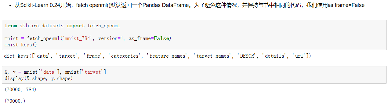
some_digit = X[0]
some_digit_image = some_digit.reshape(28, 28)
plt.imshow(some_digit_image, cmap=mpl.cm.binary)
plt.axis('off')
save_fig('some_digit_plot')
plt.show()
y = y.astype(np.uint8)
def plot_digit(data):
image = data.reshape(28, 28)
plt.imshow(image, cmap=mpl.cm.binary, interpolation='nearest') # 临近插值
plt.axis('off')
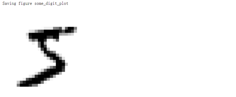
def plot_digits(instances, images_per_row=10, **options):
size = 28
images_per_row = min(len(instances), images_per_row)
images = [instance.reshape(size, size) for instance in instances]
n_rows = (len(instances) - 1) // images_per_row + 1
row_images = []
n_empty = n_rows * images_per_row - len(instances)
images.append(np.zeros((size, size * n_empty)))
for row in range(n_rows):
rimages = images[row * images_per_row : (row + 1) * images_per_row]
# 水平合并,合并列
row_images.append(np.concatenate(rimages, axis=1))
image = np.concatenate(row_images, axis=0)
plt.imshow(image, cmap=mpl.cm.binary, **options)
plt.axis('off')
plt.figure(figsize=(9, 9))
example_images = X[:100]
plot_digits(example_images, images_per_row=10)
save_fig('more_digits_plot')
plt.show()
# mnist数据集已经划分好训练集和测试集
X_train, X_test, y_train, y_test = X[:60000], X[60000:], y[:60000], y[60000:]
二分类#
y_train_5 = (y_train == 5)
y_test_5 = (y_test == 5)

from sklearn.linear_model import SGDClassifier

sgd_clf = SGDClassifier(max_iter=1000, tol=1e-3, random_state=42)  # 容差,停止迭代参数
sgd_clf.fit(X_train, y_train_5)
sgd_clf.predict([some_digit])  # array([ True])

from sklearn.model_selection import cross_val_score
# 三折
cross_val_score(sgd_clf, X_train, y_train_5, cv=3, scoring='accuracy')  # array([0.95035, 0.96035, 0.9604 ])
分层抽样#
from sklearn.model_selection import StratifiedKFold
from sklearn.base import clone

skfolds = StratifiedKFold(n_splits=3, shuffle=True, random_state=42)

for train_index, test_index in skfolds.split(X_train, y_train_5):
    clone_clf =clone(sgd_clf)
    X_train_folds = X_train[train_index]
    y_train_folds = y_train_5[train_index]
    X_test_fold = X_train[test_index]
    y_test_fold = y_train_5[test_index]

    clone_clf.fit(X_train_folds, y_train_folds)
    y_pred = clone_clf.predict(X_test_fold)
    n_correct = sum(y_pred == y_test_fold)
    print(n_correct / len(y_pred))  # 0.9669 0.91625 0.96785
准确率并不是一个好的评价指标#
from sklearn.base import BaseEstimator

class Never5Classifier(BaseEstimator):
    def fit(self, X, y=None):
        pass
    def predict(self, X):
        return np.zeros((len(X), 1), dtype=bool)

never_5_clf = Never5Classifier()
cross_val_score(never_5_clf, X_train, y_train_5, cv=3, scoring='accuracy')  # array([0.91125, 0.90855, 0.90915])
混淆矩阵:横轴实际,纵轴预测#
from sklearn.model_selection import cross_val_predict
from sklearn.metrics import confusion_matrix

y_train_pred = cross_val_predict(sgd_clf, X_train, y_train_5, cv=3)
confusion_matrix(y_train_5, y_train_pred)  # array([[53892,   687], [ 1891,  3530]])
精度/精确率#
from sklearn.metrics import precision_score, recall_score

precision_score(y_train_5, y_train_pred)  # 0.8370879772350012

cm = confusion_matrix(y_train_5, y_train_pred)
cm[1, 1] / (cm[0, 1] + cm[1, 1])  # 0.8370879772350012
召回率#
recall_score(y_train_5, y_train_pred)  # 0.6511713705958311
cm[1, 1] / (cm[1, 0] + cm[1, 1])  # 0.6511713705958311
f1#
from sklearn.metrics import f1_score

f1_score(y_train_5, y_train_pred)  # 0.7325171197343846
2 / (1/(cm[1, 1] / (cm[0, 1] + cm[1, 1])) + 1/(cm[1, 1] / (cm[1, 0] + cm[1, 1])))  # 0.7325171197343847
自定义分类阈值#
y_scores = sgd_clf.decision_function([some_digit])
y_scores  # array([2164.22030239])

threshold = 0
y_some_digit_pred = (y_scores > threshold)
y_some_digit_pred  # array([ True])

threshold = 8000
y_some_digit_pred = (y_scores > threshold)
y_some_digit_pred  # array([False])
# 默认阈值是0
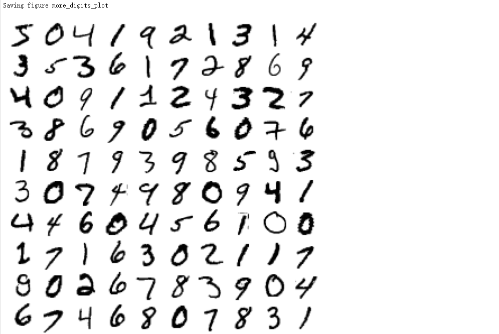
from sklearn.metrics import precision_recall_curve
y_scores = cross_val_predict(sgd_clf, X_train, y_train_5, cv=3, method='decision_function')
precisions, recalls, thresholds = precision_recall_curve(y_train_5, y_scores)
def plot_precision_recall_vs_threshold(precisions, recalls, thresholds):
plt.plot(thresholds, precisions[:-1], 'b--', label='Precision', linewidth=2)
plt.plot(thresholds, recalls[:-1], 'g-', label='Recall', linewidth=2)
plt.legend(loc='center right', fontsize=16)
plt.xlabel('Threshold', fontsize=16)
plt.grid(True)
plt.axis([-50000, 50000, 0, 1])
recall_90_precision = recalls[np.argmax(precisions >= 0.90)]
threshold_90_precision = thresholds[np.argmax(precisions >= 0.90)]
plt.figure(figsize=(8, 4))
plot_precision_recall_vs_threshold(precisions, recalls, thresholds)
plt.plot([threshold_90_precision, threshold_90_precision], [0, 0.9], 'r:')
plt.plot([-50000, threshold_90_precision], [0.9, 0.9], 'r:')
plt.plot([-50000, threshold_90_precision], [recall_90_precision, recall_90_precision], 'r:')
plt.plot([threshold_90_precision], [0.9], 'ro')
plt.plot([threshold_90_precision], [recall_90_precision], 'ro')
save_fig('precision_recall_vs_threshold_plot')
plt.show()
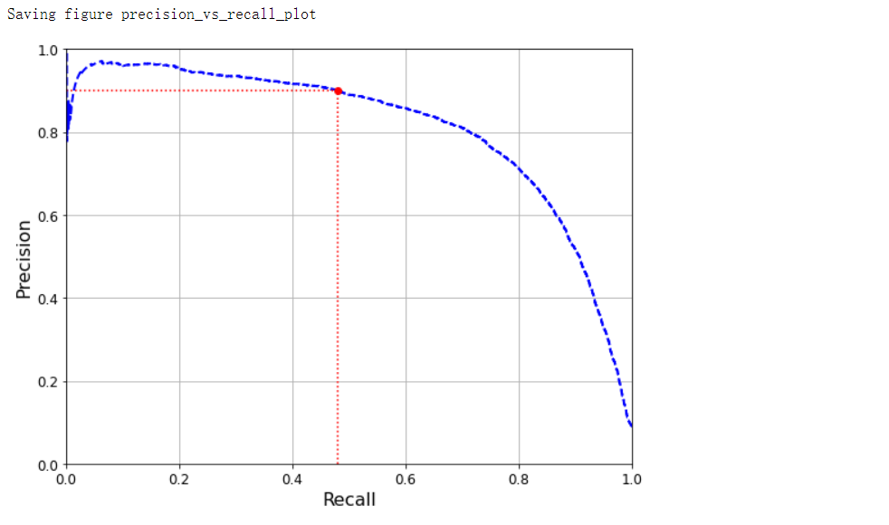
PR曲线#
def plot_precision_vs_recall(precisions, recalls):
    plt.plot(recalls, precisions, 'b--', linewidth=2)
    plt.xlabel('Recall', fontsize=16)
    plt.ylabel('Precision', fontsize=16)
    plt.axis([0, 1, 0, 1])
    plt.grid(True)

plt.figure(figsize=(8, 6))
plot_precision_vs_recall(precisions, recalls)
plt.plot([recall_90_precision, recall_90_precision], [0.0, 0.9], 'r:')
plt.plot([0.0, recall_90_precision], [0.9, 0.9], 'r:')
plt.plot([recall_90_precision], [0.9], 'ro')
save_fig('precision_vs_recall_plot')
plt.show()

# 自定义阈值
# 满足条件第一个下标
threshold_90_precision = thresholds[np.argmax(precisions >= 0.90)]
threshold_90_precision  # 3370.0194991439557

y_train_pred_90 = (y_scores >= threshold_90_precision)
precision_score(y_train_5, y_train_pred_90)  # 0.9000345901072293

recall_score(y_train_5, y_train_pred_90)  # 0.4799852425751706
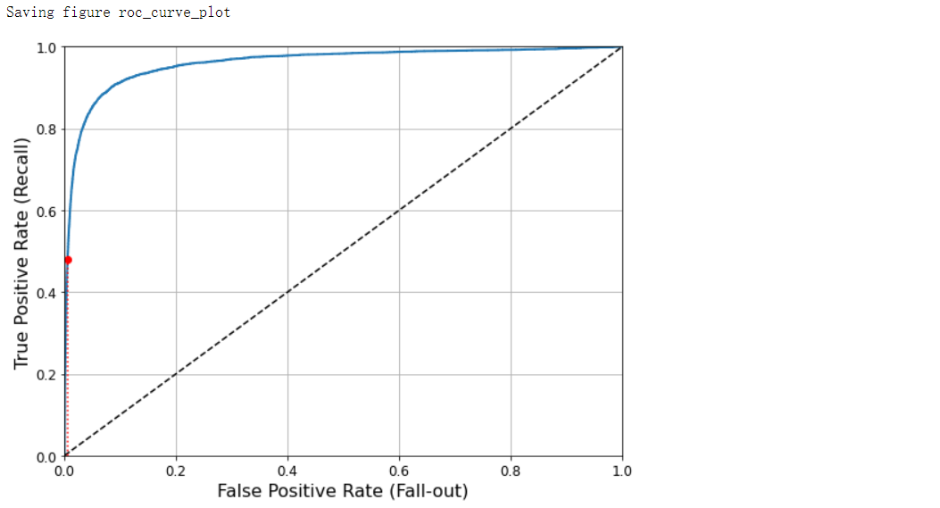
ROC曲线#
from sklearn.metrics import roc_curve

fpr, tpr, thresholds = roc_curve(y_train_5, y_scores)
def plot_roc_curve(fpr, tpr, label=None):
    plt.plot(fpr, tpr, linewidth=2, label=label)
    plt.plot([0, 1], [0, 1], 'k--')
    plt.axis([0, 1, 0, 1])
    plt.xlabel('False Positive Rate (Fall-out)', fontsize=16)
    plt.ylabel('True Positive Rate (Recall)', fontsize=16)
    plt.grid(True)

plt.figure(figsize=(8, 6))
plot_roc_curve(fpr, tpr)
fpr_90 = fpr[np.argmax(tpr >= recall_90_precision)]
plt.plot([fpr_90, fpr_90], [0.0, recall_90_precision], 'r:')
plt.plot([0.0, fpr_90], [recall_90_precision, recall_90_precision], 'r:')
plt.plot([fpr_90], [recall_90_precision], 'ro')
save_fig('roc_curve_plot')
plt.show()
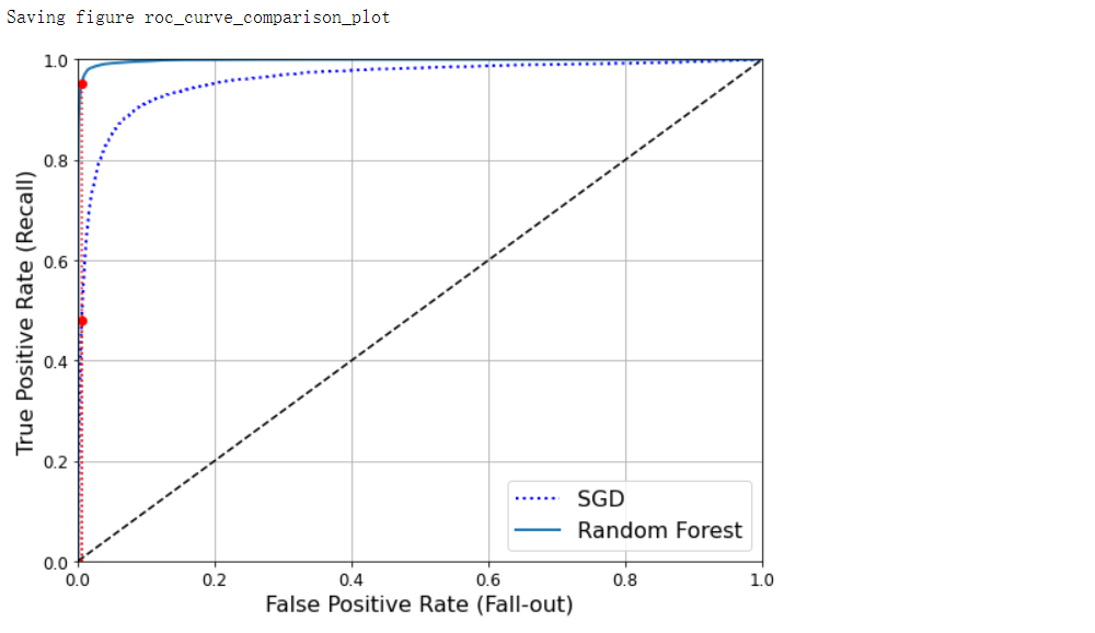
AUC#
from sklearn.metrics import roc_auc_score
from sklearn.ensemble import RandomForestClassifier

roc_auc_score(y_train_5, y_scores)
forest_clf = RandomForestClassifier(n_estimators=100, random_state=42)
y_probas_forest = cross_val_predict(forest_clf, X_train, y_train_5, cv=3, method='predict_proba')
# 得分为预测为正例的概率
y_score_forest = y_probas_forest[:, 1]
fpr_forest, tpr_forest, thresholds_forest = roc_curve(y_train_5, y_score_forest)

recall_for_forest = tpr_forest[np.argmax(fpr_forest >= fpr_90)]
plt.figure(figsize=(8, 6))
plt.plot(fpr, tpr, 'b:', linewidth=2, label='SGD')
plot_roc_curve(fpr_forest, tpr_forest, 'Random Forest')
plt.plot([fpr_90, fpr_90], [0.0, recall_90_precision], 'r:')
plt.plot([0.0, fpr_90], [recall_90_precision, recall_90_precision], 'r:')
plt.plot([fpr_90], [recall_90_precision], 'ro')
plt.plot([fpr_90, fpr_90], [0.0, recall_for_forest], 'r:')
plt.plot([fpr_90], [recall_for_forest], 'ro')
plt.grid(True)
plt.legend(loc='lower right', fontsize=16)
save_fig('roc_curve_comparison_plot')
plt.show()

roc_auc_score(y_train_5, y_score_forest)  # 0.9983436731328145

y_train_pred_forest = cross_val_predict(forest_clf, X_train, y_train_5, cv=3)
precision_score(y_train_5, y_train_pred_forest)  # 0.9905083315756169

recall_score(y_train_5, y_train_pred_forest)  # 0.8662608374838591
多分类#
from sklearn.multiclass import OneVsRestClassifier

ovr_clf = OneVsRestClassifier(SVC(gamma='auto', random_state=42))
ovr_clf.fit(X_train[:1000], y_train[:1000])
ovr_clf.predict([some_digit])

len(ovr_clf.estimators_)  # 10
标准化提升准确率#
cross_val_score(sgd_clf, X_train, y_train, cv=3, scoring='accuracy')  # array([0.87365, 0.85835, 0.8689 ])

from sklearn.preprocessing import StandardScaler
scaler = StandardScaler()
X_train_scaled = scaler.fit_transform(X_train.astype(np.float64))
cross_val_score(sgd_clf, X_train_scaled, y_train, cv=3, scoring='accuracy')  # array([0.8983, 0.891 , 0.9018])
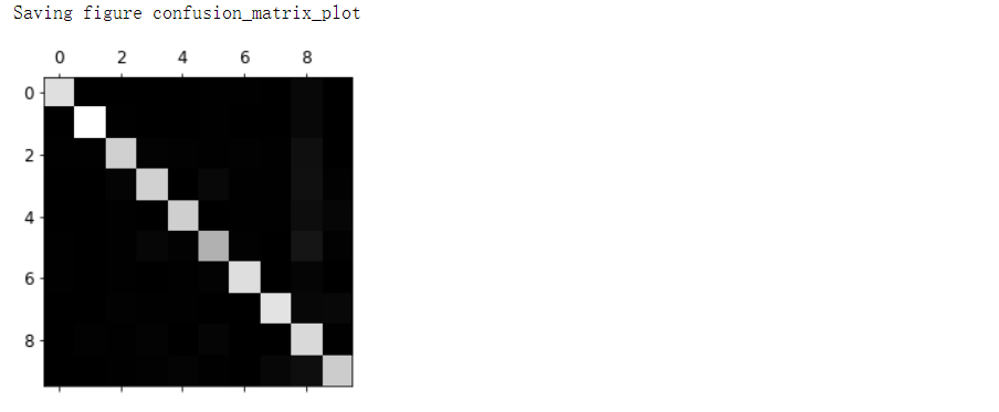
错误分析#
y_train_pred = cross_val_predict(sgd_clf, X_train_scaled, y_train, cv=3)
conf_mx = confusion_matrix(y_train, y_train_pred)
conf_mx
'''
array([[5577,    0,   22,    5,    8,   43,   36,    6,  225,    1],
       [   0, 6400,   37,   24,    4,   44,    4,    7,  212,   10],
       [  27,   27, 5220,   92,   73,   27,   67,   36,  378,   11],
       [  22,   17,  117, 5227,    2,  203,   27,   40,  403,   73],
       [  12,   14,   41,    9, 5182,   12,   34,   27,  347,  164],
       [  27,   15,   30,  168,   53, 4444,   75,   14,  535,   60],
       [  30,   15,   42,    3,   44,   97, 5552,    3,  131,    1],
       [  21,   10,   51,   30,   49,   12,    3, 5684,  195,  210],
       [  17,   63,   48,   86,    3,  126,   25,   10, 5429,   44],
       [  25,   18,   30,   64,  118,   36,    1,  179,  371, 5107]])
'''

# 彩色&colorbar
def plot_confusion_matrix(matrix):
    fig = plt.figure(figsize=(8, 8))
    ax = fig.add_subplot(111)
    cax = ax.matshow(matrix)
    fig.colorbar(cax)

plt.matshow(conf_mx, cmap=plt.cm.gray)
save_fig('confusion_matrix_plot', tight_layout=False)
plt.show()
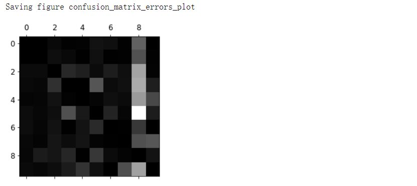
row_sums = conf_mx.sum(axis=1, keepdims=True)
norm_conf_mx = conf_mx / row_sums
# 预测为数字8的错误较多
np.fill_diagonal(norm_conf_mx, 0)
plt.matshow(norm_conf_mx, cmap=plt.cm.gray)
save_fig('confusion_matrix_errors_plot', tight_layout=False)
plt.show()
多标签分类#
from sklearn.neighbors import KNeighborsClassifier

y_train_large = (y_train >= 7)
y_train_odd = (y_train % 2 == 1)
y_multilabel = np.c_[y_train_large, y_train_odd]

knn_clf = KNeighborsClassifier()
knn_clf.fit(X_train, y_multilabel)

knn_clf.predict([some_digit])  # array([[False,  True]])

y_train_knn_pred = cross_val_predict(knn_clf, X_train, y_multilabel, cv=3)
f1_score(y_multilabel, y_train_knn_pred, average='macro')  # 0.976410265560605
多输出分类#
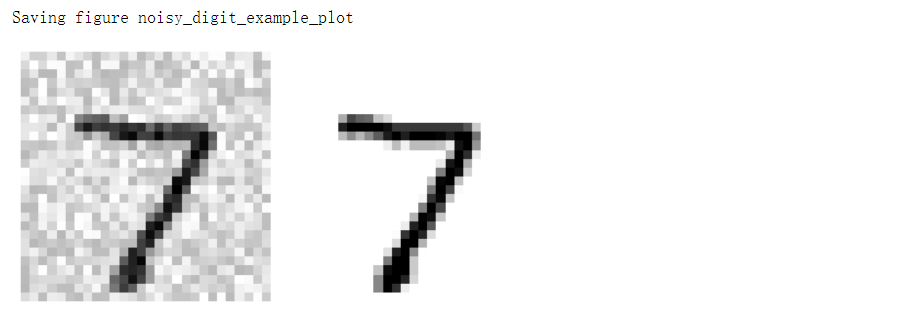
noise = np.random.randint(0, 100, (len(X_train), 784))
X_train_mod = X_train + noise
noise = np.random.randint(0, 100, (len(X_test), 784))
X_test_mod = X_test + noise
y_train_mod = X_train  # 一个y是一个输出系列
y_test_mod = X_test

some_index = 0
plt.subplot(121); plot_digit(X_test_mod[some_index])
plt.subplot(122); plot_digit(y_test_mod[some_index])
save_fig('noisy_digit_example_plot')
plt.show()
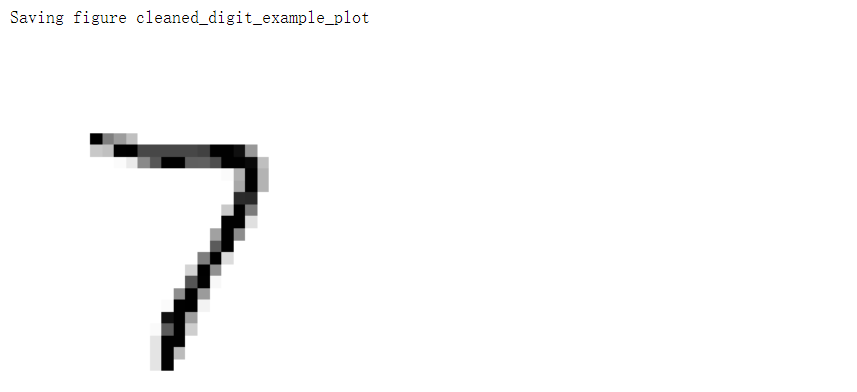
knn_clf.fit(X_train_mod, y_train_mod)
clean_digit = knn_clf.predict([X_test_mod[some_index]])
plot_digit(clean_digit)
save_fig('cleaned_digit_example_plot')
作者:lotuslaw
出处:https://www.cnblogs.com/lotuslaw/p/15533057.html
版权:本作品采用「署名-非商业性使用-相同方式共享 4.0 国际」许可协议进行许可。


【推荐】国内首个AI IDE,深度理解中文开发场景,立即下载体验Trae
【推荐】编程新体验,更懂你的AI,立即体验豆包MarsCode编程助手
【推荐】抖音旗下AI助手豆包,你的智能百科全书,全免费不限次数
【推荐】轻量又高性能的 SSH 工具 IShell:AI 加持,快人一步
· 开发者必知的日志记录最佳实践
· SQL Server 2025 AI相关能力初探
· Linux系列:如何用 C#调用 C方法造成内存泄露
· AI与.NET技术实操系列(二):开始使用ML.NET
· 记一次.NET内存居高不下排查解决与启示
· 阿里最新开源QwQ-32B,效果媲美deepseek-r1满血版,部署成本又又又降低了!
· 开源Multi-agent AI智能体框架aevatar.ai,欢迎大家贡献代码
· Manus重磅发布:全球首款通用AI代理技术深度解析与实战指南
· 被坑几百块钱后,我竟然真的恢复了删除的微信聊天记录!
· 没有Manus邀请码?试试免邀请码的MGX或者开源的OpenManus吧