
1、加载包和数据
- numpy is the fundamental package for scientific computing with Python.
- h5py is a common package to interact with a dataset that is stored on an H5 file.
- matplotlib is a famous library to plot graphs in Python.
- PIL and scipy are used here to test your model with your own picture at the end
__author__ = 'Qian Chenglong'

import numpy as np
import matplotlib.pyplot as plt
import h5py
import scipy
from scipy import ndimage
from lr_utils import load_dataset

#load data
train_set_x_orig, train_set_y, test_set_x_orig, test_set_y, classes = load_dataset()
2、处理数据
1)看一下数据的形状
#get she shape of thed data
print(train_set_x_orig.shape)
print(train_set_y.shape)
print(test_set_x_orig.shape)
print(test_set_y.shape)
print(classes.shape)
2)获取训练数据个数和测试数据个数,图片是64*64*3的格式
#the number of data,train number is 209 test number is50
m_train = train_set_x_orig.shape[0]
m_test = test_set_x_orig.shape[0]

#the picture's row * col =64*64 channel=3
num_px = train_set_x_orig.shape[1]
3)重构数据形状
A trick when you want to flatten a matrix X of shape (a,b,c,d) to a matrix X_flatten of shape (b∗c∗d, a) is to use:
X_flatten = X.reshape(X.shape[0], -1).T # X.T is the transpose of X
train_set_x_flatten = train_set_x_orig.reshape(train_set_x_orig.shape[0], -1).T
test_set_x_flatten = test_set_x_orig.reshape(test_set_x_orig.shape[0], -1).T
4)标准化(归一化)处理数据,因为图片的数据都是0~255的所以我们直接/255
# standardize our dataset.
train_set_x = train_set_x_flatten/255.
test_set_x = test_set_x_flatten/255.
5)定义要使用的函数
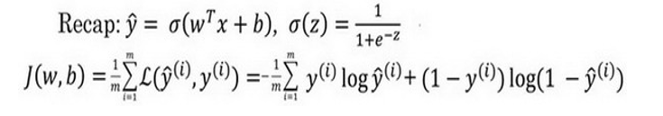
sigmoid函数在这里被称为激活函数。 𝑠𝑖𝑔𝑚𝑜𝑖𝑑(z)=1+(1+exp(-z))
def sigmoid(z):
    s=1/(1+np.exp(-z))
    return s
初始化函数(注意,在多神经元的神经网络中,w必须采用随机初始化,b可以采用zero初始化)
#dim: the number of features
def initialize_with_zeros(dim):
    w=np.zeros((dim,1))
    b=0
    assert (w.shape == (dim, 1))    #assert()判断()条件是否为真,为假会报错
    assert (isinstance(b, float) or isinstance(b, int))
    return w,b
正向传播函数:(loss函数选择的交叉熵函数=𝑦(𝑖)log(𝑎(𝑖))+(1−𝑦(𝑖))log(1−𝑎(𝑖))),其中a(i)是网络的输出,与下面公式中的a不是同一个)

a是学习率
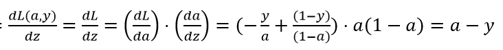
注意:这里的a已经变成了神经元的输出y_hat
对于单个数据样本使用loss函数进行更新,
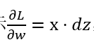 ,
,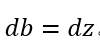
但也可以同时使用多个样本更新,即使用cost函数更新

   """
    Implement the cost function and its gradient for the propagation explained above

    Arguments:
    w -- weights, a numpy array of size (num_px * num_px * 3, 1)
    b -- bias, a scalar
    X -- data of size (num_px * num_px * 3, number of examples)
    Y -- true "label" vector (containing 0 if non-cat, 1 if cat) of size (1, number of examples)

    Return:
    cost -- negative log-likelihood cost for logistic regression
    dw -- gradient of the loss with respect to w, thus same shape as w
    db -- gradient of the loss with respect to b, thus same shape as b

    """
def propagate(w, b, X, Y):

    m = X.shape[1]        #get the number of the data
    A=sigmoid((np.dot(w.T,X)+b))   # compute activation
    cost = -1 / m * np.sum(Y * np.log(A) + (1 - Y) * np.log(1 - A))   # compute cost

    dw = 1 / m * np.dot(X, (A - Y).T)
    db = 1 / m * np.sum(A - Y)

    assert (dw.shape == w.shape)
    assert (db.dtype == float)
    cost = np.squeeze(cost)  # 压缩矩阵形状,删除多余的维度
    assert (cost.shape == ())

    grads = {"dw": dw,
             "db": db}

    return grads, cost
#
优化器(反向传播函数)
  """
    This function optimizes w and b by running a gradient descent algorithm

    Arguments:
    w -- weights, a numpy array of size (num_px * num_px * 3, 1)
    b -- bias, a scalar
    X -- data of shape (num_px * num_px * 3, number of examples)
    Y -- true "label" vector (containing 0 if non-cat, 1 if cat), of shape (1, number of examples)
    num_iterations -- number of iterations of the optimization loop
    learning_rate -- learning rate of the gradient descent update rule
    print_cost -- True to print the loss every 100 steps

    Returns:
    params -- dictionary containing the weights w and bias b
    grads -- dictionary containing the gradients of the weights and bias with respect to the cost function
    costs -- list of all the costs computed during the optimization, this will be used to plot the learning curve.

    """
def optimize(w, b, X, Y, num_iterations, learning_rate, print_cost=False):


    costs = []

    for i in range(num_iterations):

        grads, cost = propagate(w, b, X, Y)
        # Retrieve derivatives from grads
        dw = grads["dw"]
        db = grads["db"]

        # update rule
        w = w - learning_rate * dw
        b = b - learning_rate * db

        # Record the costs
        if i % 100 == 0:
            costs.append(cost)

        # Print the cost every 100 training examples
        if print_cost and i % 100 == 0:
            print ("Cost after iteration %i: %f" % (i, cost))

    params = {"w": w,
              "b": b}

    grads = {"dw": dw,
             "db": db}

    return params, grads, costs
预测函数
  '''
    Predict whether the label is 0 or 1 using learned logistic regression parameters (w, b)

    Arguments:
    w -- weights, a numpy array of size (num_px * num_px * 3, 1)
    b -- bias, a scalar
    X -- data of size (num_px * num_px * 3, number of examples)

    Returns:
    Y_prediction -- a numpy array (vector) containing all predictions (0/1) for the examples in X
    '''
def predict(w, b, X):
    m = X.shape[1]
    Y_prediction = np.zeros((1, m))
    w = w.reshape(X.shape[0], 1)

    # Compute vector "A" predicting the probabilities of a cat being present in the picture
    A = sigmoid(np.dot(w.T, X) + b)

    for i in range(A.shape[1]):

        # Convert probabilities A[0,i] to actual predictions p[0,i]
        if A[0, i] <= 0.5:
            Y_prediction[0, i] = 0
        else:
            Y_prediction[0, i] = 1


    assert (Y_prediction.shape == (1, m))

    return Y_prediction
模型调用函数
   """
    Builds the logistic regression model by calling the function you've implemented previously

    Arguments:
    X_train -- training set represented by a numpy array of shape (num_px * num_px * 3, m_train)
    Y_train -- training labels represented by a numpy array (vector) of shape (1, m_train)
    X_test -- test set represented by a numpy array of shape (num_px * num_px * 3, m_test)
    Y_test -- test labels represented by a numpy array (vector) of shape (1, m_test)
    num_iterations -- hyperparameter representing the number of iterations to optimize the parameters
    learning_rate -- hyperparameter representing the learning rate used in the update rule of optimize()
    print_cost -- Set to true to print the cost every 100 iterations

    Returns:
    d -- dictionary containing information about the model.
    """
def model(X_train, Y_train, X_test, Y_test, num_iterations=2000, learning_rate=0.5, print_cost=False):
    # initialize parameters with zeros (≈ 1 line of code)
    w, b = initialize_with_zeros(X_train.shape[0])

    # Gradient descent (≈ 1 line of code)
    parameters, grads, costs = optimize(w, b, X_train, Y_train, num_iterations, learning_rate, print_cost)

    # Retrieve parameters w and b from dictionary "parameters"
    w = parameters["w"]
    b = parameters["b"]

    # Predict test/train set examples (≈ 2 lines of code)
    Y_prediction_test = predict(w, b, X_test)
    Y_prediction_train = predict(w, b, X_train)

    # Print train/test Errors
    print("train accuracy: {} %".format(100 - np.mean(np.abs(Y_prediction_train - Y_train)) * 100))
    print("test accuracy: {} %".format(100 - np.mean(np.abs(Y_prediction_test - Y_test)) * 100))

    d = {"costs": costs,
         "Y_prediction_test": Y_prediction_test,
         "Y_prediction_train": Y_prediction_train,
         "w": w,
         "b": b,
         "learning_rate": learning_rate,
         "num_iterations": num_iterations}

    return d
调用模型
d = model(train_set_x, train_set_y, test_set_x, test_set_y, num_iterations = 2000, learning_rate = 0.005, print_cost = True)
画出cost的曲线
# Plot learning curve (with costs)
costs = np.squeeze(d['costs'])
plt.plot(costs)
plt.ylabel('cost')
plt.xlabel('iterations (per hundreds)')
plt.title("Learning rate =" + str(d["learning_rate"]))
plt.show()

learning_rates = [0.01, 0.001, 0.0001]
models = {}
for i in learning_rates:
    print ("learning rate is: " + str(i))
    models[str(i)] = model(train_set_x, train_set_y, test_set_x, test_set_y, num_iterations = 1500, learning_rate = i, print_cost = False)
    print ('\n' + "-------------------------------------------------------" + '\n')

for i in learning_rates:
    plt.plot(np.squeeze(models[str(i)]["costs"]), label= str(models[str(i)]["learning_rate"]))

plt.ylabel('cost')
plt.xlabel('iterations')

legend = plt.legend(loc='upper center', shadow=True)
frame = legend.get_frame()
frame.set_facecolor('0.90')
plt.show()
使用自己的图片测试
my_image = "cat_in_iran.jpg"   # change this to the name of your image file


# We preprocess the image to fit your algorithm.
fname = "images/" + my_image
image = np.array(ndimage.imread(fname, flatten=False))
my_image = scipy.misc.imresize(image, size=(num_px,num_px)).reshape((1, num_px*num_px*3)).T
my_predicted_image = predict(d["w"], d["b"], my_image)

plt.imshow(image)
print("y = " + str(np.squeeze(my_predicted_image)) + ", your algorithm predicts a \"" + classes[
完整代码
lr_utils.py
import numpy as np
import h5py


def load_dataset():
    train_dataset = h5py.File(r'F:\TensorFlow_practice\TensorFlow\NNmindset\datasets\train_catvnoncat.h5', "r")
    train_set_x_orig = np.array(train_dataset["train_set_x"][:])  # your train set features
    train_set_y_orig = np.array(train_dataset["train_set_y"][:])  # your train set labels

    test_dataset = h5py.File(r'F:\TensorFlow_practice\TensorFlow\NNmindset\datasets\test_catvnoncat.h5', "r")
    test_set_x_orig = np.array(test_dataset["test_set_x"][:])  # your test set features
    test_set_y_orig = np.array(test_dataset["test_set_y"][:])  # your test set labels

    classes = np.array(test_dataset["list_classes"][:])  # the list of classes

    train_set_y_orig = train_set_y_orig.reshape((1, train_set_y_orig.shape[0]))
    test_set_y_orig = test_set_y_orig.reshape((1, test_set_y_orig.shape[0]))

    return train_set_x_orig, train_set_y_orig, test_set_x_orig, test_set_y_orig, classes
single_nerve_network.py
__author__ = 'Qian Chenglong'

import numpy as np
import matplotlib.pyplot as plt
import h5py
import scipy
from scipy import ndimage
from lr_utils import load_dataset

#load data
train_set_x_orig, train_set_y, test_set_x_orig, test_set_y, classes = load_dataset()

# index = 5
# plt.imshow(train_set_x_orig[index])
# print ("y = " + str(train_set_y[:, index]) + ", it's a '" + classes[np.squeeze(train_set_y[:, index])].decode("utf-8") +  "' picture.")

#get she shape of thed data
print(train_set_x_orig.shape)
print(train_set_y.shape)
print(test_set_x_orig.shape)
print(test_set_y.shape)
print(classes.shape)


#the number of data,train number is 209 test number is50
m_train = train_set_x_orig.shape[0]
m_test = test_set_x_orig.shape[0]

#the picture's row * col =64*64
num_px = train_set_x_orig.shape[1]

#
train_set_x_flatten = train_set_x_orig.reshape(train_set_x_orig.shape[0], -1).T
test_set_x_flatten = test_set_x_orig.reshape(test_set_x_orig.shape[0], -1).T


# standardize our dataset.
train_set_x = train_set_x_flatten/255.
test_set_x = test_set_x_flatten/255.


def sigmoid(z):
    s=1/(1+np.exp(-z))
    return s

#dim: the number of features
def initialize_with_zeros(dim):
    w=np.zeros((dim,1))
    b=0
    assert (w.shape == (dim, 1))    #assert()判断()条件是否为真,为假会报错
    assert (isinstance(b, float) or isinstance(b, int))
    return w,b

"""
    Implement the cost function and its gradient for the propagation explained above

    Arguments:
    w -- weights, a numpy array of size (num_px * num_px * 3, 1)
    b -- bias, a scalar
    X -- data of size (num_px * num_px * 3, number of examples)
    Y -- true "label" vector (containing 0 if non-cat, 1 if cat) of size (1, number of examples)

    Return:
    cost -- negative log-likelihood cost for logistic regression
    dw -- gradient of the loss with respect to w, thus same shape as w
    db -- gradient of the loss with respect to b, thus same shape as b

    """
def propagate(w, b, X, Y):

    m = X.shape[1]        #get the number of the data
    A=sigmoid((np.dot(w.T,X)+b))   # compute activation
    cost = -1 / m * np.sum(Y * np.log(A) + (1 - Y) * np.log(1 - A))   # compute cost

    dw = 1 / m * np.dot(X, (A - Y).T)
    db = 1 / m * np.sum(A - Y)

    assert (dw.shape == w.shape)
    assert (db.dtype == float)
    cost = np.squeeze(cost)  # 压缩矩阵形状,删除多余的维度
    assert (cost.shape == ())

    grads = {"dw": dw,
             "db": db}

    return grads, cost

"""
    This function optimizes w and b by running a gradient descent algorithm

    Arguments:
    w -- weights, a numpy array of size (num_px * num_px * 3, 1)
    b -- bias, a scalar
    X -- data of shape (num_px * num_px * 3, number of examples)
    Y -- true "label" vector (containing 0 if non-cat, 1 if cat), of shape (1, number of examples)
    num_iterations -- number of iterations of the optimization loop
    learning_rate -- learning rate of the gradient descent update rule
    print_cost -- True to print the loss every 100 steps

    Returns:
    params -- dictionary containing the weights w and bias b
    grads -- dictionary containing the gradients of the weights and bias with respect to the cost function
    costs -- list of all the costs computed during the optimization, this will be used to plot the learning curve.

    """
def optimize(w, b, X, Y, num_iterations, learning_rate, print_cost=False):
    costs = []

    for i in range(num_iterations):

        grads, cost = propagate(w, b, X, Y)
        # Retrieve derivatives from grads
        dw = grads["dw"]
        db = grads["db"]

        # update rule
        w = w - learning_rate * dw
        b = b - learning_rate * db

        # Record the costs
        if i % 100 == 0:
            costs.append(cost)

        # Print the cost every 100 training examples
        if print_cost and i % 100 == 0:
            print ("Cost after iteration %i: %f" % (i, cost))

    params = {"w": w,
              "b": b}

    grads = {"dw": dw,
             "db": db}

    return params, grads, costs

    '''
    Predict whether the label is 0 or 1 using learned logistic regression parameters (w, b)

    Arguments:
    w -- weights, a numpy array of size (num_px * num_px * 3, 1)
    b -- bias, a scalar
    X -- data of size (num_px * num_px * 3, number of examples)

    Returns:
    Y_prediction -- a numpy array (vector) containing all predictions (0/1) for the examples in X
    '''
def predict(w, b, X):
    m = X.shape[1]
    Y_prediction = np.zeros((1, m))
    w = w.reshape(X.shape[0], 1)

    # Compute vector "A" predicting the probabilities of a cat being present in the picture
    A = sigmoid(np.dot(w.T, X) + b)

    for i in range(A.shape[1]):

        # Convert probabilities A[0,i] to actual predictions p[0,i]
        if A[0, i] <= 0.5:
            Y_prediction[0, i] = 0
        else:
            Y_prediction[0, i] = 1


    assert (Y_prediction.shape == (1, m))

    return Y_prediction

    """
    Builds the logistic regression model by calling the function you've implemented previously

    Arguments:
    X_train -- training set represented by a numpy array of shape (num_px * num_px * 3, m_train)
    Y_train -- training labels represented by a numpy array (vector) of shape (1, m_train)
    X_test -- test set represented by a numpy array of shape (num_px * num_px * 3, m_test)
    Y_test -- test labels represented by a numpy array (vector) of shape (1, m_test)
    num_iterations -- hyperparameter representing the number of iterations to optimize the parameters
    learning_rate -- hyperparameter representing the learning rate used in the update rule of optimize()
    print_cost -- Set to true to print the cost every 100 iterations

    Returns:
    d -- dictionary containing information about the model.
    """
def model(X_train, Y_train, X_test, Y_test, num_iterations=2000, learning_rate=0.5, print_cost=False):
    # initialize parameters with zeros (≈ 1 line of code)
    w, b = initialize_with_zeros(X_train.shape[0])

    # Gradient descent (≈ 1 line of code)
    parameters, grads, costs = optimize(w, b, X_train, Y_train, num_iterations, learning_rate, print_cost)

    # Retrieve parameters w and b from dictionary "parameters"
    w = parameters["w"]
    b = parameters["b"]

    # Predict test/train set examples (≈ 2 lines of code)
    Y_prediction_test = predict(w, b, X_test)
    Y_prediction_train = predict(w, b, X_train)

    # Print train/test Errors
    print("train accuracy: {} %".format(100 - np.mean(np.abs(Y_prediction_train - Y_train)) * 100))
    print("test accuracy: {} %".format(100 - np.mean(np.abs(Y_prediction_test - Y_test)) * 100))

    d = {"costs": costs,
         "Y_prediction_test": Y_prediction_test,
         "Y_prediction_train": Y_prediction_train,
         "w": w,
         "b": b,
         "learning_rate": learning_rate,
         "num_iterations": num_iterations}

    return d

d = model(train_set_x, train_set_y, test_set_x, test_set_y, num_iterations = 2000, learning_rate = 0.005, print_cost = True)

# Example of a picture that was wrongly classified.
index = 1
plt.imshow(test_set_x[:,index].reshape((num_px, num_px, 3)))
print ("y = " + str(test_set_y[0,index]) + ", you predicted that it is a \"" + classes[int(d["Y_prediction_test"][0,index])].decode("utf-8") +  "\" picture.")

# Plot learning curve (with costs)
costs = np.squeeze(d['costs'])
plt.plot(costs)
plt.ylabel('cost')
plt.xlabel('iterations (per hundreds)')
plt.title("Learning rate =" + str(d["learning_rate"]))
plt.show()

learning_rates = [0.01, 0.001, 0.0001]
models = {}
for i in learning_rates:
    print ("learning rate is: " + str(i))
    models[str(i)] = model(train_set_x, train_set_y, test_set_x, test_set_y, num_iterations = 1500, learning_rate = i, print_cost = False)
    print ('\n' + "-------------------------------------------------------" + '\n')

for i in learning_rates:
    plt.plot(np.squeeze(models[str(i)]["costs"]), label= str(models[str(i)]["learning_rate"]))

plt.ylabel('cost')
plt.xlabel('iterations')

legend = plt.legend(loc='upper center', shadow=True)
frame = legend.get_frame()
frame.set_facecolor('0.90')
plt.show()

 浙公网安备 33010602011771号