结合w2v与svm对酒店评论数据进行情感倾向分析

数据集：ChnSentiCorp-Htl-ba-4000

由于该数据集中的文件是分散的（一句评论一个文件），这样处理起来会比较麻烦，所以我们先要对它们进行合并：

# 这个步骤建议在本地完成，因为colab读取大量零散的google drive文件的速度非常慢

from tqdm import tqdm

def combine_files(data_label, dir_path):
  data_files = os.listdir(dir_path)
  data_collection = []
  for data_file in tqdm(data_files):
    with open(dir_path + '//' + data_file, "r", encoding='utf-8') as file_pipeline:
      data = file_pipeline.read()
      data_collection.append(data)
  with open(data_label + '.pickle', 'rb') as file_pipeline:
    pickle.dump(data_collection, file_pipeline)

接下来，我们进行数据预处理，这里包含了字符过滤，去停用词，分词等三个步骤：

这里使用的停用词表为：四川大学机器智能实验室停用词库 scu_stopwords.txt

# 注意neg.1156.txt中的评论内容过少，经停用词处理后得到空字符串

import os
import re
import pickle
import jieba
from tqdm import tqdm

DATA_DIR = "/content/drive/Shared drives/A/data/ChnSentiCorp/ChnSentiCorp-Htl-ba-4000/"
NEG_DATA_DIR = DATA_DIR + "neg.pickle"
POS_DATA_DIR = DATA_DIR + "pos.pickle"
STOPWORDS_PATH = "/content/drive/Shared drives/A/data/stopwords/scu_stopwords.txt"

# 只保留中文字符
def clean_data(data):
  data = data.replace('\n', '')
  data = re.sub(r'[a-zA-Z0-9]', '', data)
  data = re.sub(r"[\s+\.\!\/_,$%^*(+\"\']+|[+—！，。？?;；、~@#￥%…&*（）]+", "", data)
  return data

# 分词
def cut_sentence(data, stopwords):
  word_list = jieba.cut(data)
  result = []
  for word in word_list:
    if word not in stopwords:
      result.append(word)
  return ' '.join(result).strip()

# 去除停用词
def get_stopwords(stopwords_path):
  with open(stopwords_path, 'r', encoding='utf8') as file_pipeline:
    data = file_pipeline.read()
    data = set(data.strip().split('\n'))
  return data

# 读取并处理数据
def process_data(data_path, stopwords):
  data_collection = []
  with open(data_path, 'rb') as file_pipeline:
    contents = pickle.load(file_pipeline)
    for index, content in tqdm(enumerate(contents)):
      data = clean_data(content)
      data = cut_sentence(data, stopwords)
      data_collection.append(data)
  return data_collection

# 分别处理正负样本，保存处理结果
stopwords = get_stopwords(STOPWORDS_PATH)
neg_data = process_data(NEG_DATA_DIR, stopwords)
pos_data = process_data(POS_DATA_DIR, stopwords)
with open(DATA_DIR + 'neg_cleaned.pickle','wb') as file_pipeline:
  pickle.dump(neg_data, file_pipeline)
with open(DATA_DIR + 'pos_cleaned.pickle','wb') as file_pipeline:
  pickle.dump(pos_data, file_pipeline)

接下来我们要把文本数据转化成向量数据，这里用到了上一篇博客中训练的词向量模型：

import pickle
import numpy as np
import pandas as pd
from tqdm import tqdm
from gensim.models import Word2Vec

# 把一组词转化为一组词向量
def get_word_vecs(word_list, model):
  vecs = []
  for word in word_list:
    word = word.replace('\n', '')
    try:
      vecs.append(model[word])
    except KeyError:
      continue
  return np.array(vecs, dtype='float')

# 构建句子向量
def build_vecs(data_path, model):
  doc_vecs = []
  with open(data_path, 'rb') as file_pipeline:
    contents = pickle.load(file_pipeline)
    for index, line in tqdm(enumerate(contents)):
      word_list = line.split(' ')
      word_vecs = get_word_vecs(word_list, model)
      # 用句子中所有词向量的均值来表示这个句子
      if len(word_vecs) > 0:
        sentence_vec = np.mean(word_vecs, axis=0)
        doc_vecs.append(sentence_vec)
  return doc_vecs

# 加载预训练词向量模型
data_dir = '/content/drive/Shared drives/A/data/ChnSentiCorp/ChnSentiCorp-Htl-ba-4000/'
w2v_model_path = '/content/drive/Shared drives/A/data/pre_training/wiki_zh_w2v/wiki_zh_text_model'
w2v_model = Word2Vec.load(w2v_model_path).wv

# 数据向量化
posInput = build_vecs(data_dir + 'pos_cleaned.pickle', w2v_model)
negInput = build_vecs(data_dir + 'neg_cleaned.pickle', w2v_model)

# 数据标签：1-pos, 0-neg
Y = np.concatenate((np.ones(len(posInput)), np.zeros(len(negInput))))
X = np.array(posInput + negInput)

# 保存结果 
df_x = pd.DataFrame(X)
df_y = pd.DataFrame(Y)
result = pd.concat([df_y,df_x],axis = 1)
print(result)
result.to_csv(data_dir + 'vec_data.csv')

最后是降维与分类：

# 降维与分类

import numpy as np
import pandas as pd
import matplotlib.pyplot as plt
from sklearn.decomposition import PCA
from sklearn import svm, metrics
from sklearn.model_selection import GridSearchCV, train_test_split

data_dir = '/content/drive/Shared drives/A/data/ChnSentiCorp/ChnSentiCorp-Htl-ba-4000/'

# 读取数据
df = pd.read_csv(data_dir + 'vec_data.csv')
y = df.iloc[:,1]
x = df.iloc[:,2:]

# 分析降维范围
n_components = 400
pca = PCA(n_components=n_components)
pca.fit(x)

plt.figure(1, figsize=(4, 3))
plt.clf()
plt.axes([.2, .2, .7, .7])
plt.plot(pca.explained_variance_, linewidth=2)
plt.axis('tight')
plt.xlabel('n_components')
plt.ylabel('explained_variance_')
plt.show()

# 降维
x_pca = PCA(n_components = 100).fit_transform(x)

# 将数据划分为训练集和测试集，test_size=.2表示20%的测试集
x_train, x_test, y_train, y_test = train_test_split(x_pca, y, test_size=.2)

# svm分类并测试
svc = svm.SVC(kernel='rbf', class_weight='balanced',)
c_range = np.logspace(-5, 15, 11, base=2)
gamma_range = np.logspace(-9, 3, 13, base=2)

# 网格搜索交叉验证的参数范围，cv=3,3折交叉
param_grid = [{'kernel': ['rbf'], 'C': c_range, 'gamma': gamma_range}]
grid = GridSearchCV(svc, param_grid, cv=3, n_jobs=-1)

# 训练模型
clf = grid.fit(x_train, y_train)

# 计算测试集精度
score = grid.score(x_test, y_test)
print('精度为%s' % score)

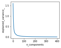
通过由pca.explained_variance_绘制出的图像可以看出，前100维的向量已经具备较高的区分能力，因此我们把400维的词向量压缩至100维，然后喂入svm进行训练，最后得到的精度为：88.1%