第二周学习

线性回归

本节主要学习了采用线性模型进行数据拟合，来达到与预测的效果。

# 简单演示pytorch求导的方法
import torch
x = torch.tensor(3.0, requires_grad=False)
# print(x.requires_grad)
# x.requires_grad_()
# print(x.requires_grad)
y = 2*x
y.requires_grad_()
z = y**2
f = z+2
f.backward()
print(y.is_leaf)
print(x.grad)
print(y.grad)
print(z.grad)

# 导入所需的工具包
%matplotlib inline
import random
import torch
from d2l import torch as d2l

# 生产数据集并附加噪声
def synthetic_data(w, b, num_examples):
    X = torch.normal(0, 1, (num_examples, len(w)))
    Y = torch.matmul(X, w) + b
    Y += torch.normal(0, 0.01, Y.shape)
    return X, Y.reshape((-1, 1))

true_w = torch.tensor([2, -3.4])
true_b = 4.2
features, labels = synthetic_data(true_w, true_b, 1000)
print('features:', features[0], '\nlabel:', labels[0])
d2l.set_figsize()
d2l.plt.scatter(features[:, 1].detach().numpy(), labels.detach().numpy(), 1)

# 读取数据集
def data_iter(batch_size, features, labels):
    num_examples = len(features)
    indices = list(range(num_examples))

    random.shuffle(indices)
    for i in range(0, num_examples, batch_size):
        batch_indices = torch.tensor(indices[i: min(i+batch_size, num_examples)])
        yield features[batch_indices], labels[batch_indices]

batch_size = 10
for X, Y in data_iter(batch_size, features, labels):
    print(X, '\n', Y)
    break
    
# 初始化超参数 w，b
w = torch.normal(0, 0.01, size=(2, 1), requires_grad=True)
b = torch.zeros(1, requires_grad=True)

# 定义线性函数
def linreg(X, w, b):
    return torch.matmul(X, w) + b

# 定义损失函数
def squared_loss(y_hat, y):
    return (y_hat-y.reshape(y_hat.shape))**2/2

# 采用随机梯度下降进行优化
def sgd(params, lr, batch_size):
    with torch.no_grad():
        for param in params:
            param -= lr * param.grad/batch_size
            param.grad.zero_()
            
# 进行训练
lr = 0.01
num_epochs = 50
net  = linreg
loss = squared_loss
for epoch in range(num_epochs):
    for X, Y in data_iter(batch_size, features, labels):
        l = loss(net(X, w, b), Y)
        l.sum().backward()
        sgd([w, b], lr, batch_size)
    with torch.no_grad():
        train_l = loss(net(features, w, b), labels)
        print(f'epoch {epoch + 1}, loss {float(train_l.mean()):f}')
        
print(f'w的估计误差：{true_w - w.reshape(true_w.shape)}')
print(f'w的估计误差：{true_b - b}')

# 借助 pytorch 提供的函数实现线性回归

# 导入所需的工具包
import numpy as np
import torch
from torch import nn
from torch.utils import data
from d2l import torch as d2l

# 生成并加载数据集
true_w = torch.tensor([2, -3.4])
true_b = 4.2
features, labels = d2l.synthetic_data(true_w, true_b, 1000)
def load_array(data_array, batch_size, is_train=True):
    dataset = data.TensorDataset(*data_array)
    return data.DataLoader(dataset, batch_size, shuffle = is_train)

batch_size = 10
data_iter = load_array((features, labels), batch_size)

next(iter(data_iter))

# 定义网络模型，选择 pytorch 自带的线性回归函数 
net = nn.Sequential(nn.Linear(2, 1))

# 初始化参数
net[0].weight.data.normal_(0, 0.01)
net[0].bias.data.fill_(0)

# 定义损失函数
loss = nn.MSELoss()

# 定义优化器
trainer = torch.optim.SGD(net.parameters(), lr=0.03)

# 进行训练
num_epochs = 3
for epoch in range(num_epochs):
    for X, Y in data_iter:
        l = loss(net(X), Y)
        trainer.zero_grad()
        l.backward()
        trainer.step()
    l = loss(net(features), labels)
    print(f'epoch{epoch+1}, loss{l:f}')

Softmax 回归

本节主要讲解了使用 Softmax 回归进行数据的预测

# 导入常用的工具包
%matplotlib inline
import torch
import torchvision
from torch.utils import data
from torchvision import transforms
from d2l import torch as d2l

d2l.use_svg_display()

# 通过ToTensor实例将图像数据从PIL类型变换成32位浮点数格式
# 并除以255使得所有像素的数值均在0到1之间
trans = transforms.ToTensor()
mnist_train = torchvision.datasets.FashionMNIST(root="../data", train=True, transform=trans, download=True)
mnist_test = torchvision.datasets.FashionMNIST(root="../data", train=False, transform=trans, download=True)
len(mnist_train), len(mnist_test)
mnist_train[0][0].shape

# 定义返回数据集标签的函数
def get_fashion_mnist_labels(labels):
    # 返回Fashion-MNIST数据集的文本标签
    text_labels = ['t-shirt', 'trouser', 'pullover', 'dress', 'coat', 'sandal', 						'shirt', 'sneaker', 'bag', 'ankle boot']
    return [text_labels[int(i)] for i in labels]

# 定义可视化图片的函数
def show_images(imgs, num_rows, num_cols, titles=None, scale=1.5):
    figsize = (num_cols * scale, num_rows * scale)
    _, axes = d2l.plt.subplots(num_rows, num_cols, figsize=figsize)
    axes = axes.flatten()
    for i, (ax, img) in enumerate(zip(axes, imgs)):
        if torch.is_tensor(img):
            # 图片张量
            ax.imshow(img.numpy())
        else:
            # PIL图片
            ax.imshow(img)
        ax.axes.get_xaxis().set_visible(False)
        ax.axes.get_yaxis().set_visible(False)
        if titles:
            ax.set_title(titles[i])
    return axes

# 加载数据并显示图片
X, y = next(iter(data.DataLoader(mnist_train, batch_size=18)))
print(len(y))
show_images(X.reshape(18, 28, 28), 2, 9, titles=get_fashion_mnist_labels(y))

# 小批量读取数据
batch_size = 256

def get_dataloader_workers():
    return 4

train_iter = data.DataLoader(mnist_test, batch_size, shuffle=True, num_workers=get_dataloader_workers())

timer = d2l.Timer()
for X, y in train_iter:
    continue

f'{timer.stop() :.2f} sec'

# 定义下载 Fashion-MNIST 数据集，并将其加载到内存中的函数
def load_data_fashion_mnist(batch_size, resize=None):
    
    trans = [transforms.ToTensor()]
    
    if resize:
        trans.insert(0, transforms.Resize(resize))
    
    trans = transforms.Compose(trans)
    mnist_train = torchvision.datasets.FashionMNIST(root='../data', train=True, 
                                                    transform=trans, download=True)
    mnist_test = torchvision.datasets.FashionMNIST(root='../data', trian=False, 
                                                   transform=trans, download=True)

    return (data.DataLoader(mnist_train, batch_size, shuffle=True, 	
                            num_workers=get_dataloader_workers()),
        data.DataLoader(mnist_test, batch_size, shuffle=False,
                        num_workers=get_dataloader_workers()))

# 采用 Softmax 回归进行预测

# 导入需要的包
import torch
from IPython import display
from d2l import torch as d2l

# 批量读取数据集
batch_size = 256
train_iter, test_iter = d2l.load_data_fashion_mnist(batch_size)

# 初始化参数
num_inputs = 784
num_outputs = 10

W = torch.normal(0, 0.01, size=(num_inputs, num_outputs), requires_grad=True)
b = torch.zeros(num_outputs, requires_grad=True)

# 定义 Softmax 函数
def softmax(X):
    X_exp = torch.exp(X)
    partition = X_exp.sum(1, keepdim=True)
    return X_exp/partition

X = torch.normal(0, 1, (2, 5))
X_prob = softmax(X)
X_prob, X_prob.sum(1)

# 定义网络模型
def net(X):
    return softmax(torch.matmul(X.reshape(-1, W.shape[0]), W) + b)

# 定义损失函数
y = torch.tensor([0, 2])
y_hat = torch.tensor([[0.1, 0.3, 0.6], [0.3, 0.2, 0.5]])
y_hat[[0, 1], y]

def cross_entropy(y_hat, y):
    return -torch.log(y_hat[range(len(y_hat)), y])

cross_entropy(y_hat, y)

# 计算正确预测个数的函数
def accurancy(y_hat, y):
    if len(y_hat.shape) > 1 and y_hat.shape[1] > 1:
        y_hat = y_hat.argmax(axis=1)
    cmp = y_hat.type(y.dtype) == y
    return float(cmp.type(y.dtype).sum())

# 计算准确率的函数
def evaluate_accuracy(net, data_iter):
    # 计算在指定数据集上模型的精度
    if isinstance(net, torch.nn.Module):
        net.eval() # 将模型设置为评估模式
    metric = Accumulator(2) # 正确预测数、预测总数
    for X, y in data_iter:
        metric.add(accurancy(net(X), y), y.numel())
    return metric[0] / metric[1]

# 储存正确预测个数和预测个数的类
class Accumulator:
    def __init__(self, n):
        self.data = [0.0] * n
    
    def add(self, *args):
        self.data = [a + float(b) for a, b in zip(self.data, args)]

    def reset(self):
        self.data = [0.0] * len(self.data)
    
    def __getitem__(self, idx):
        return self.data[idx]

class Animator:
    def __init__(self, xlabel=None, ylabel=None, legend=None, 
            xlim=None, ylim=None, xscale='linear', yscale='linear', 
            fmts=('-', 'm--', 'g-.', 'r:'), nrows=1, ncols=1, 
            figsize=(3.5, 2.5)):
        if legend is None:
            legend = []
        d2l.use_svg_display()
        self.fig, self.axes = d2l.plt.subplots(nrows, ncols, figsize=figsize)
        if nrows * ncols == 1:
            self.axes = [self.axes, ]
        self.config_axes = lambda: d2l.set_axes(
            self.axes[0], xlabel, ylabel, xlim, ylim, xscale, yscale, legend)
        self.X, self.Y, self.fmts = None, None, fmts
    
    def add(self, x, y):
        if not hasattr(y, "__len__"):
            y = [y]
        n = len(y)
        if not hasattr(x, "__len__"):
            x = [x] * n
        if not self.X:
            self.X = [[] for _ in range(n)]
        if not self.Y:
            self.Y = [[] for _ in range(n)]
        for i, (a, b) in enumerate(zip(x, y)):
            if a is not None and b is not None:
                self.X[i].append(a)
                self.Y[i].append(b)
        self.axes[0].cla()
        for x, y, fmt in zip(self.X, self.Y, self.fmts):
            self.axes[0].plot(x, y, fmt)
        self.config_axes()
        display.display(self.fig)
        display.clear_output(wait=True)

evaluate_accuracy(net, test_iter)


# 定义进行一轮训练的函数
def train_epoch_ch3(net, tran_iter, loss, updater):
    if isinstance(net, torch.nn.Module):
        net.train()
    metric = Accumulator(3)
    for X, y in train_iter:
        y_hat = net(X)
        l = loss(y_hat, y)
        if isinstance(updater, torch.optim.Optimizer):
            updater.zero_grad()
            l.backward()
            updater.step()
            metric.add(float(l) * len(y), accurancy(y_hat, y), y.size().numel())
        else:
            l.sum().backward()
            updater(X.shape[0])
            metric.add(float(l.sum()), accurancy(y_hat, y), y.numel())
    
    return metric[0] / metric[2], metric[1] / metric[2] 

# 定义训练函数
def train_ch3(net, train_iter, test_iter, loss, num_epochs, updater):
    animator = Animator(xlabel='epoch', xlim=[1, num_epochs], ylim=[0.3, 0.9], 
                        legend=['train loss', 'train acc', 'test acc'])
    for epoch in range(num_epochs):
        train_metrics = train_epoch_ch3(net, train_iter, loss, updater)
        test_acc = evaluate_accuracy(net, test_iter)
        animator.add(epoch + 1, train_metrics + (test_acc, ))
    train_loss, train_acc = train_metrics
    assert train_loss < 0.5, train_loss
    assert train_acc <= 1 and train_acc > 0.7, train_acc
    assert test_acc <= 1 and test_acc > 0.7, test_acc

lr = 0.1
# 定义优化器
def updater(batch_size):
    return d2l.sgd([W, b], lr, batch_size)

# 进行训练
num_epochs = 10
train_ch3(net, train_iter, test_iter, cross_entropy, num_epochs, updater)

# 定义预测函数
def predict_ch3(net, test_iter, n=6):
    for X, y in test_iter:
       break
    trues = d2l.get_fashion_mnist_labels(y) 
    preds = d2l.get_fashion_mnist_labels(net(X).argmax(axis=1))
    titles = [true + '\n' + pred for true, pred in zip(trues, preds)]
    d2l.show_images(X[0:n].reshape((n, 28, 28)), 1, n, titles=titles[0:n])

# 进行预测
predict_ch3(net, test_iter)

# 借助 pytorch 内部函数实现Softmax 回归

# 导入所需的工具包
import torch
from torch import nn
from d2l import torch as d2l

# 加载数据
batch_size = 256
train_iter, test_iter = d2l.load_data_fashion_mnist(batch_size)

# 定义网络并初始化参数
net = nn.Sequential(nn.Flatten(), nn.Linear(784, 10))

def init_weights(m):
    if type(m) == nn.Linear:
        nn.init.normal_(m.weight, std=0.01)

net.apply(init_weights)

# 定义损失函数
loss = nn.CrossEntropyLoss()

# 定义优化器
trainer = torch.optim.SGD(net.parameters(), lr=0.1)

# 进行训练
num_epochs = 10
d2l.train_ch3(net, train_iter, test_iter, loss, num_epochs, trainer)

多层感知机

本节主要讲了采用多层感知机解决了线性回归不能解决非线性问题的缺点，主要是通过模拟人类的神经元，引入了激活函数，使问题得到解决

# 导入工具包并加载数据集
import torch
from torch import nn
from d2l import torch as d2l

batch_size = 256
train_iter, test_iter = d2l.load_data_fashion_mnist(batch_size)

# 初始化参数
num_inputs, num_outputs, num_hiddens = 784, 10, 256

W1 = nn.Parameter(torch.randn(num_inputs, num_hiddens, requires_grad=True) * 0.01)
b1 = nn.Parameter(torch.zeros(num_hiddens, requires_grad=True))
W2 = nn.Parameter(torch.randn(num_hiddens, num_outputs, requires_grad=True) * 0.01)
b2 = nn.Parameter(torch.zeros(num_outputs, requires_grad=True))

params = [W1, b1, W2, b2]

# 定义激活函数
def relu(X):
    a = torch.zeros_like(X)
    return torch.max(X, a)

# 定义网络
def net(X):
    X = X.reshape((-1, num_inputs))
    H = relu(X @ W1 + b1)
    return (H @ W2 + b2)

# 定义损失函数
loss = nn.CrossEntropyLoss()

# 进行训练
num_epochs, lr = 10, 0.1
updater = torch.optim.SGD(params, lr=lr)
d2l.train_ch3(net, train_iter, test_iter, loss, num_epochs, updater)

# 通过调用 pytorch 的内部函数实现多层感知机

# 导入常见的工具包
import torch
from torch import nn
from d2l import torch as d2l

# 定义网络结构
net = nn.Sequential(nn.Flatten(), nn.Linear(784, 256), nn.ReLU(), nn.Linear(256, 10))

# 定义初始化参数函数
def init_weights(m):
    if type(m) == nn.Linear:
        nn.init.normal_(m.weight, std = 0.01)

net.apply(init_weights)

# 定义损失函数和优化器
batch_size, lr, num_epochs = 256, 0.1, 10
loss = nn.CrossEntropyLoss()
trainer = torch.optim.SGD(net.parameters(), lr=lr)

# 进行训练
train_iter, test_iter = d2l.load_data_fashion_mnist(batch_size)
d2l.train_ch3(net, train_iter, test_iter, loss, num_epochs, trainer)

过拟合和欠拟合

本节主要讲了模型选择中应该要注意的问题和过拟合、欠拟合

# 导入工具包
import math
import numpy as np
import torch
from torch import nn
from d2l import torch as d2l

# 生成数据集
max_degree = 20
n_train, n_test = 100, 100
true_w = np.zeros(max_degree)
true_w[0:4] = np.array([5, 1.2, -3.4, 5.6])

features = np.random.normal(size=(n_train + n_test, 1))
np.random.shuffle(features)
poly_features = np.power(features, np.arange(max_degree).reshape(1, -1))
for i in range(max_degree):
    poly_features[:, i] /= math.gamma(i + 1)
labels = np.dot(poly_features, true_w)
labels += np.random.normal(scale=0.1, size=labels.shape)

true_w, features, poly_features, labels = [
    torch.tensor(x, dtype=torch.float32)
    for x in [true_w, features, poly_features, labels]]

features[:2], poly_features[:2, :], labels[:2]

# 损失评估函数
def evaluate_loss(net, data_iter, loss):
    # 评估给定数据集上模型的损失
    metric = d2l.Accumulator(2)
    for X, y in data_iter:
        out = net(X)
        y = y.reshape(out.shape)
        l = loss(out, y)
        metric.add(l.sum(), l.numel())
    return metric[0] / metric[1]

# 定义训练函数
def train(train_features, test_features, train_labels, test_labels, num_epochs=400):
    loss = nn.MSELoss()
    input_shape = train_features.shape[-1]
    net = nn.Sequential(nn.Linear(input_shape, 1, bias=False))
    batch_size = min(10, train_labels.shape[0])
    train_iter = d2l.load_array((train_features, train_labels.reshape(-1, 1)), 
                                batch_size)
    test_iter = d2l.load_array((test_features, test_labels.reshape(-1, 1)), 
                               batch_size, is_train=False)
    trainer = torch.optim.SGD(net.parameters(), lr=0.01)
    animator = d2l.Animator(xlabel='epoch', ylabel='loss', yscale='log', 
                            xlim=[1, num_epochs], ylim=[1e-3, 1e2], 
                            legend=['train', 'test'])
    for epoch in range(num_epochs):
        d2l.train_epoch_ch3(net, train_iter, loss, trainer)
        if epoch == 0 or (epoch + 1) % 20 == 0:
            animator.add(epoch+1, (evaluate_loss(net, train_iter, loss), 
                                   evaluate_loss(net, test_iter, loss)))
    print('weight:', net[0].weight.data.numpy())
    
# 采用三阶多项式拟合
train(poly_features[:n_train, :4], poly_features[n_train:, :4], 
      labels[:n_train], labels[n_train:])

# 采用线性拟合（欠拟合）
train(poly_features[:n_train, :2], poly_features[n_train:, :2], 
      labels[:n_train], labels[n_train:])

# 采用二十阶多项式拟合（过拟合）
train(poly_features[:n_train, :], poly_features[n_train:, :], 
      labels[:n_train], labels[n_train:])

权重衰退

本节主要讲解了通过权重衰退的方式缓解过拟合

# 导入工具包
%matplotlib inline
import torch
from torch import nn
from d2l import torch as d2l

# 生产并加载数据集
n_train, n_test, num_inputs, batch_size = 20, 100, 200, 5
true_w, true_b = torch.ones((num_inputs, 1)) * 0.01, 0.05
train_data = d2l.synthetic_data(true_w, true_b, n_train)
train_iter = d2l.load_array(train_data, batch_size)
test_data = d2l.synthetic_data(true_w, true_b, n_test)
test_iter = d2l.load_array(test_data, batch_size, is_train=False)

# 初始化参数
def init_params():
    w = torch.normal(0, 1, size=(num_inputs, 1), requires_grad=True)
    b = torch.zeros(1, requires_grad=True)
    return [w, b]

# 定义 L1、L2 范数
def l2_penalty(w):
    return torch.sum(w.pow(2))/2

def l1_penalty(w):
    return torch.sum(torch.abs(w))

# 定义训练函数
def train(lambd):
    w, b = init_params()
    net, loss = lambda X: d2l.linreg(X, w, b), d2l.squared_loss
    num_epochs, lr = 100, 0.003
    animator = d2l.Animator(xlabel='epochs', ylabel='loss', yscale='log', 
                            xlim=[5, num_epochs], legend=['train', 'test'])
    for epoch in range(num_epochs):
        for X, y in train_iter:
            # with torch.enable_grad():
            l = loss(net(X), y) + lambd * l2_penalty(w)
            l.sum().backward()
            d2l.sgd([w, b], lr, batch_size)
        if (epoch + 1) % 5 == 0:
            animator.add(epoch + 1, (d2l.evaluate_loss(net, train_iter, loss), 
                                     d2l.evaluate_loss(net, test_iter, loss)))
    print('w的L2范数是：', torch.norm(w).item())

# 进行训练
train(lambd=0)

train(lambd=3)

# 借助 pytorch 工具类实现权重衰退

# 定义训练函数
def train_concise(wd):
    net = nn.Sequential(nn.Linear(num_inputs, 1))
    for param in net.parameters():
        param.data.normal_()
    loss = nn.MSELoss()
    num_epochs, lr = 100, 0.003
    # weight_decay 为权重衰退的权重 lambda
    trainer = torch.optim.SGD([{"params": net[0].weight, "weight_decay": wd}, 
                               {"params": net[0].bias}], lr=lr)
    animator = d2l.Animator(xlabel='epoch', ylabel='loss', yscale='log', 
                            xlim=[5, num_epochs], legend=['train', 'test'])
    for epoch in range(num_epochs):
        for X, y in train_iter:
            with torch.enable_grad():
                trainer.zero_grad()
                l = loss(net(X), y)
            l.backward()
            trainer.step()
        if (epoch + 1) % 5 == 0:
            animator.add(epoch+1, (d2l.evaluate_loss(net, train_iter, loss),
                                   d2l.evaluate_loss(net, test_iter, loss)))
    print('w的L2范数：', net[0].weight.norm().item())
    
# 进行训练
train_concise(wd=0)

train_concise(wd=3)

Dropout

本节主要讲解了通过 Dropout 的方法缓解过拟合

# 导入需要的工具包
import torch
from torch import nn
from d2l import torch as d2l

# 定义Dropout函数
def dropout_layer(X, dropout):
    assert 0 <= dropout <= 1
    if dropout == 1:
        return torch.zeros_like(X)
    if dropout == 0:
        return X
    mask = (torch.Tensor(X.shape).uniform_(0, 1) > dropout).float()
    return mask * X / (1.0 - dropout)

X = torch.arange(16, dtype=torch.float32).reshape((2, 8))
print(X)
print(dropout_layer(X, 0.))
print(dropout_layer(X, 0.5))
print(dropout_layer(X, 1.0))

# 定义网络模型
class Net(nn.Module):
    def __init__(self, num_inputs, num_outputs, num_hiddens1, num_hiddens2, is_training=True):
        super(Net, self).__init__()
        self.num_inputs = num_inputs
        self.training = is_training
        self.lin1 = nn.Linear(num_inputs, num_hiddens1)
        self.lin2 = nn.Linear(num_hiddens1, num_hiddens2)
        self.lin3 = nn.Linear(num_hiddens2, num_outputs)
        self.relu = nn.ReLU()

    def forward(self, X):
        H1 = self.relu(self.lin1(X.reshape(-1, num_inputs)))
        if self.training == True:
            H1 = dropout_layer(H1, dropout1)
        H2 = self.relu(self.lin2(H1))
        if self.training == True:
            H2 = dropout_layer(H2, dropout2)
        out = self.lin3(H2)
        return out

num_inputs, num_outputs, num_hiddens1, num_hiddens2 = 784, 10, 256, 256
dropout1, dropout2 = 0.2, 0.5

net = Net(num_inputs, num_outputs, num_hiddens1, num_hiddens2)

# 初始化参数
num_epochs, lr, batch_size = 10, 0.5, 256

# 定义损失函数
loss = nn.CrossEntropyLoss()

# 加载数据集
train_iter, test_iter = d2l.load_data_fashion_mnist(batch_size)

# 定义优化器
trainer = torch.optim.SGD(net.parameters(), lr=lr)

# 进行训练
d2l.train_ch3(net, train_iter, test_iter, loss, num_epochs, trainer)

# 借助 pytorch 内部函数实现 Dropout

# 定义网络
net = nn.Sequential(nn.Flatten(), nn.Linear(784, 256), nn.ReLU(), 
            nn.Dropout(dropout1), nn.Linear(256, 256), nn.ReLU(), 
            nn.Dropout(dropout2), nn.Linear(256, 10))

# 初始化参数
def init_weights(m):
    if type(m) == nn.Linear:
        nn.init.normal_(m.weight, std=0.01)
net.apply(init_weights)

# 定义优化器
trainer = torch.optim.SGD(net.parameters(), lr=lr)

# 进行训练
d2l.train_ch3(net, train_iter, test_iter, loss, num_epochs, trainer)

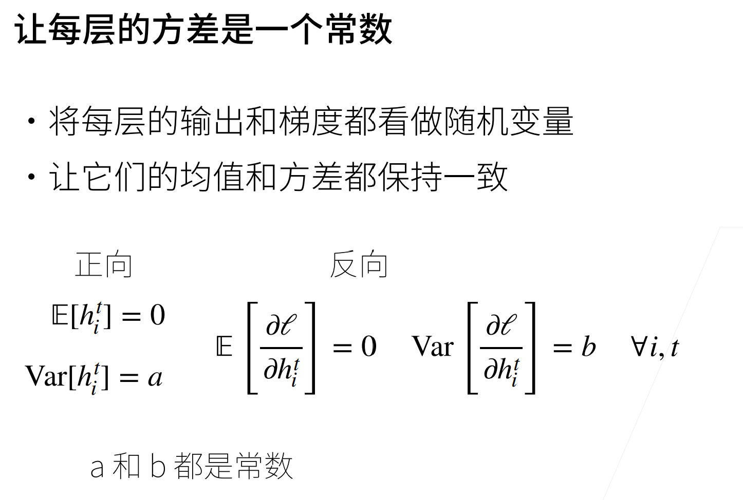
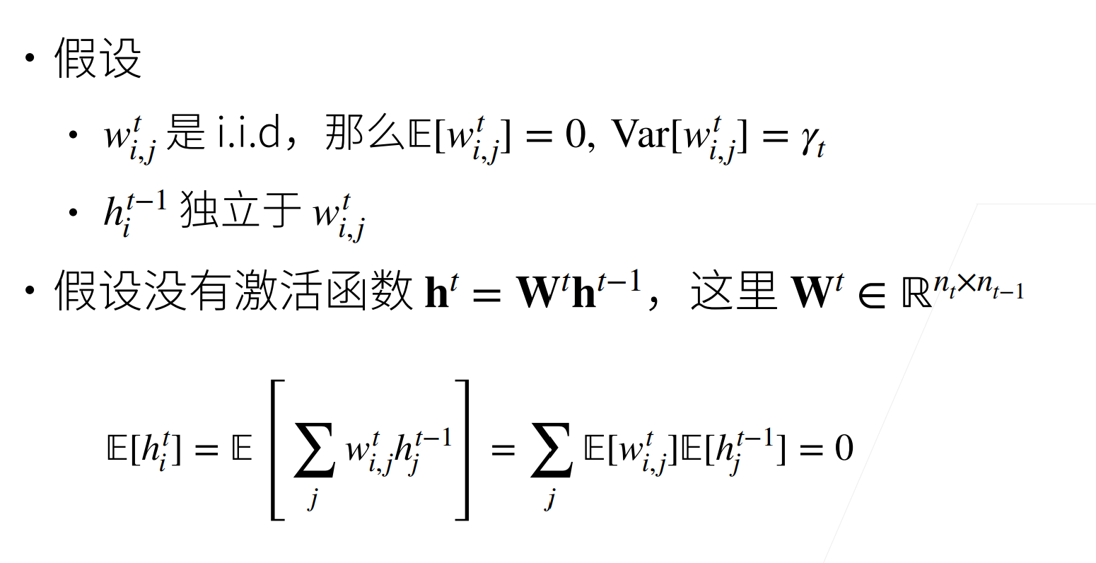
数值稳定性、模型评估和激活函数

本节主要讲解了在训练过程中可能会出现的梯度爆炸和梯度消失问题

# 导入工具包
%matplotlib inline
import torch
from d2l import torch as d2l

# 梯度消失
x = torch.arange(-8.0, 8.0, 0.1, requires_grad=True)
y = torch.sigmoid(x)
y.backward(torch.ones_like(x))

d2l.plot(x.detach().numpy(), [y.detach().numpy(), x.grad.numpy()],
         legend=['sigmoid', 'gradient'], figsize=(4.5, 2.5))

# 梯度爆炸
M = torch.normal(0, 1, size=(4,4))
print('一个矩阵 \n',M)
for i in range(100):
    M = torch.mm(M,torch.normal(0, 1, size=(4, 4)))

print('乘以100个矩阵后\n', M)

参数初始化不再采用默认的方式，而是使用 Xavier 初始化方法