
第四次学习
MobileNetV1
这篇文章的主要内容是采用深度可分离卷积(深度卷积+逐点卷积)实现了轻量级的网络,相比于标准卷积,其参数和计算量大幅下降,并且精度并未有很大的降低。
标准卷积
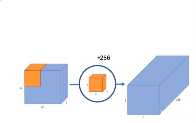
输入一个12×12×3的一个输入特征图,经过5×5×3的卷积核卷积得到一个8×8×1的输出特征图。如果此时我们有256个特征图,我们将会得到一个8×8×256的输出特征图。
深度卷积
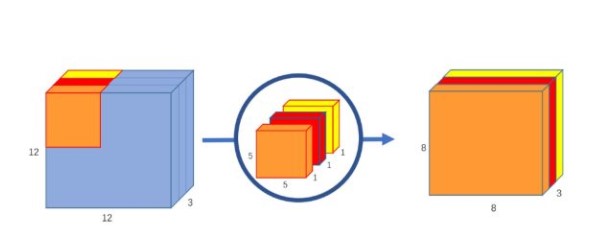
与标准卷积网络不一样的是,我们将卷积核拆分成为但单通道形式,在不改变输入特征图像的深度的情况下,对每一通道进行卷积操作,这样就得到了和输入特征图通道数一致的输出特征图。如上图:输入12×12×3的特征图,经过5×5×1×3的深度卷积之后,得到了8×8×3的输出特征图。输入个输出的维度是不变的3。
逐点卷积
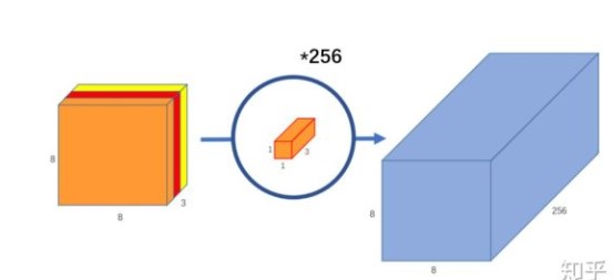
在深度卷积的过程中,我们得到了8×8×3的输出特征图,我们用256个1×1×3的卷积核对输入特征图进行卷积操作,输出的特征图和标准的卷积操作一样都是8×8×256了。
参数量与计算量对比
标准卷积的参数量与计算量
参数量:\(D_K \times D_K \times M \times N\)
计算量:\(D_K \times D_K \times M \times N \times D_W \times D_H\)
深度可分离卷积的参数量与计算量
参数量:\(D_K \times D_K \times M + M \times N\)
计算量:\(D_K \times D_K \times M \times D_W \times D_H + M \times N \times D_W \times D_H\)
比值:
参数数量和乘加操作的运算量均下降为原来的:
我们通常所使用的是3×3的卷积核,也就是会下降到原来的九分之一到八分之一
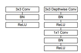
网络结构

上图左边是标准卷积层,右边是V1的卷积层。V1的卷积层,首先使用3×3的深度卷积提取特征,接着是一个BN层,随后是一个ReLU层,在之后就会逐点卷积,最后就是BN和ReLU了。这也很符合深度可分离卷积,将左边的标准卷积拆分成右边的一个深度卷积和一个逐点卷积。

MobileNet的网络结构如上图所示。首先是一个3x3的标准卷积,s2进行下采样。然后就是堆积深度可分离卷积,并且其中的部分深度卷积会利用s2进行下采样。然后采用平均池化层将feature变成1x1,根据预测类别大小加上全连接层,最后是一个softmax层。整个网络有28层,其中深度卷积层有13层。
代码练习
class Block(nn.Module):
    def __init__(self, in_planes, out_planes, stride=1):
        super(Block, self).__init__()
        self.conv1 = nn.Conv2d(in_planes, in_planes, kernel_size=3, stride=stride, padding=1, groups=in_planes, bias=False)
        self.bn1 = nn.BatchNorm2d(in_planes)
        self.conv2 = nn.Conv2d(in_planes, out_planes, kernel_size=1, stride=1, padding=0, bias=False)
        self.bn2 = nn.BatchNorm2d(out_planes)

    def forward(self, x):
        out = F.relu(self.bn1(self.conv1(x)))
        out = F.relu(self.bn2(self.conv2(out)))
        return out
创建 DataLoader
device = torch.device("cuda:0" if torch.cuda.is_available() else "cpu")

transform_train = transforms.Compose([
    transforms.RandomCrop(32, padding=4),
    transforms.RandomHorizontalFlip(),
    transforms.ToTensor(),
    transforms.Normalize((0.4914, 0.4822, 0.4465), (0.2023, 0.1994, 0.2010))
])

transform_test = transforms.Compose([
    transforms.ToTensor(),
    transforms.Normalize((0.4914, 0.4822, 0.4465), (0.2023, 0.1994, 0.2010))
])

trainset = torchvision.datasets.CIFAR10(root='./data', train=True, download=True, transform=transform_train)
testset = torchvision.datasets.CIFAR10(root='./data', train=False, download=True, transform=transform_test)

trainloader = torch.utils.data.DataLoader(trainset, batch_size=128, shuffle=True, num_workers=2)
testloader = torch.utils.data.DataLoader(testset, batch_size=128, shuffle=False, num_workers=2)
创建 MobileNetV1 网络
32×32×3 ==>
32×32×32 ==> 32×32×64 ==> 16×16×128 ==> 16×16×128 ==>
8×8×256 ==> 8×8×256 ==> 4×4×512 ==> 4×4×512 ==>
2×2×1024 ==> 2×2×1024
接下来为均值 pooling ==> 1×1×1024
最后全连接到 10个输出节点
class MobileNetV1(nn.Module):
    cfg = [(64,1), (128,2), (128,1), (256,2), (256,1), (512,2), (512,1), (1024,2), (1024,1)]

    def __init__(self, num_classes=10):
        super(MobileNetV1, self).__init__()
        self.conv1 = nn.Conv2d(3, 32, kernel_size=3, stride=1, padding=1, bias=False)
        self.bn1 = nn.BatchNorm2d(32)
        self.layers = self._make_layers(in_planes=32)
        self.linear = nn.Linear(1024, num_classes)

    def _make_layers(self, in_planes):
        layers = []
        for x in self.cfg:
            out_planes = x[0]
            stride = x[1]
            layers.append(Block(in_planes, out_planes, stride))
            in_planes = out_planes
        return nn.Sequential(*layers)

    def forward(self, x):
        out = F.relu(self.bn1(self.conv1(x)))
        out = self.layers(out)
        out = F.avg_pool2d(out, 2)
        out = out.view(out.size(0), -1)
        out = self.linear(out)
        return out
模型训练
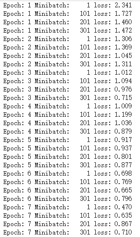
for epoch in range(10):
    for i, (inputs, labels) in enumerate(trainloader):
        inputs = inputs.to(device)
        labels = labels.to(device)

        optimizer.zero_grad()

        outputs = net(inputs)
        loss = criterion(outputs, labels)
        loss.backward()
        optimizer.step()

        if i%100 == 0:
            print('Epoch: %d Minibatch: %5d loss: %.3f' %(epoch + 1, i + 1, loss.item()))
print('Finished Training')

测试
correct = 0
total = 0

for data in testloader:
    images, labels = data
    images, labels = images.to(device), labels.to(device)
    outputs = net(images)
    _, predicted = torch.max(outputs.data, 1)
    total += labels.size(0)
    correct += (predicted == labels).sum().item()

print('Accuracy of the network on the 10000 test images: %.2f %%'%(100*correct/total))

MobileNetV2
V1核心思想是采用 深度可分离卷积 操作。在相同的权值参数数量的情况下,相较标准卷积操作,可以减少数倍的计算量,从而达到提升网络运算速度的目的。
首先利用3×3的深度可分离卷积提取特征,然后利用1×1的卷积来扩张通道。用这样的block堆叠起来的MobileNetV1既能较少不小的参数量、计算量,提高网络运算速度,又能的得到一个接近于标准卷积的还不错的结果。
但是,有人在实际使用的时候, 发现深度卷积部分的卷积核比较容易训废掉:训完之后发现深度卷积训出来的卷积核有不少是空的。
作者认为是因为对低维度做ReLU运算,很容易造成信息的丢失,而在高维度进行ReLU运算的话,信息的丢失则会很少。所以将ReLU替换成线性激活函数。
linear bottleneck
我们当然不能把所有的激活层都换成线性的啊,只是将最后的ReLU6换成Linear,作者将这个部分称之为linear bottleneck。
Expansion layer
深度卷积本身没有改变通道的能力,来的是多少通道输出就是多少通道。如果来的通道很少的话,DW深度卷积只能在低维度上工作,这样效果并不会很好,所以我们要“扩张”通道。作者使用PW卷积进行升维(升维倍数为t,t=6),再在一个更高维的空间中进行卷积操作来提取特征:
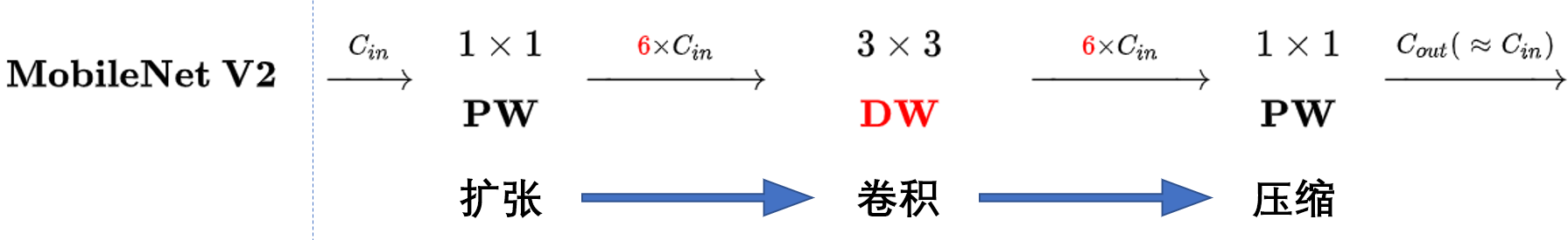
也就是说,不管输入通道数是多少,经过第一个PW逐点卷积升维之后,深度卷积都是在相对的更高6倍维度上进行工作。
Inverted residuals
我们希望像Resnet一样复用我们的特征,所以我们引入了shortcut结构,这样V2的block就是如下图形式:
对比一下ResNet和MobileNetV2
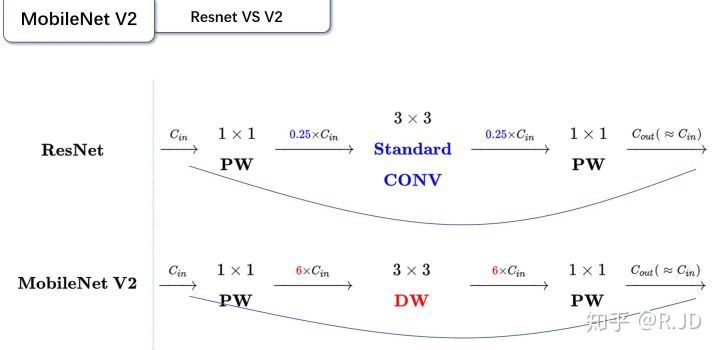
可以发现,都采用了 1×1 -> 3 ×3 -> 1 × 1 的模式,以及都使用Shortcut结构。但是不同点在于:
- ResNet 先降维 (0.25倍)、卷积、再升维。
- MobileNetV2 则是 先升维 (6倍)、卷积、再降维。
刚好V2的block刚好与Resnet的block相反,作者将其命名为Inverted residuals。
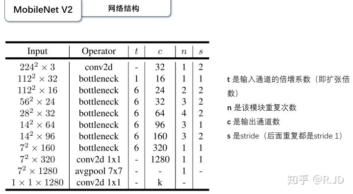
网络结构
Block

对比一下V1和V2
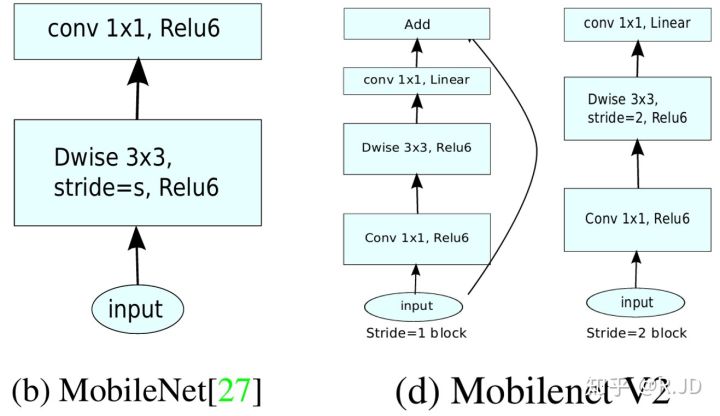
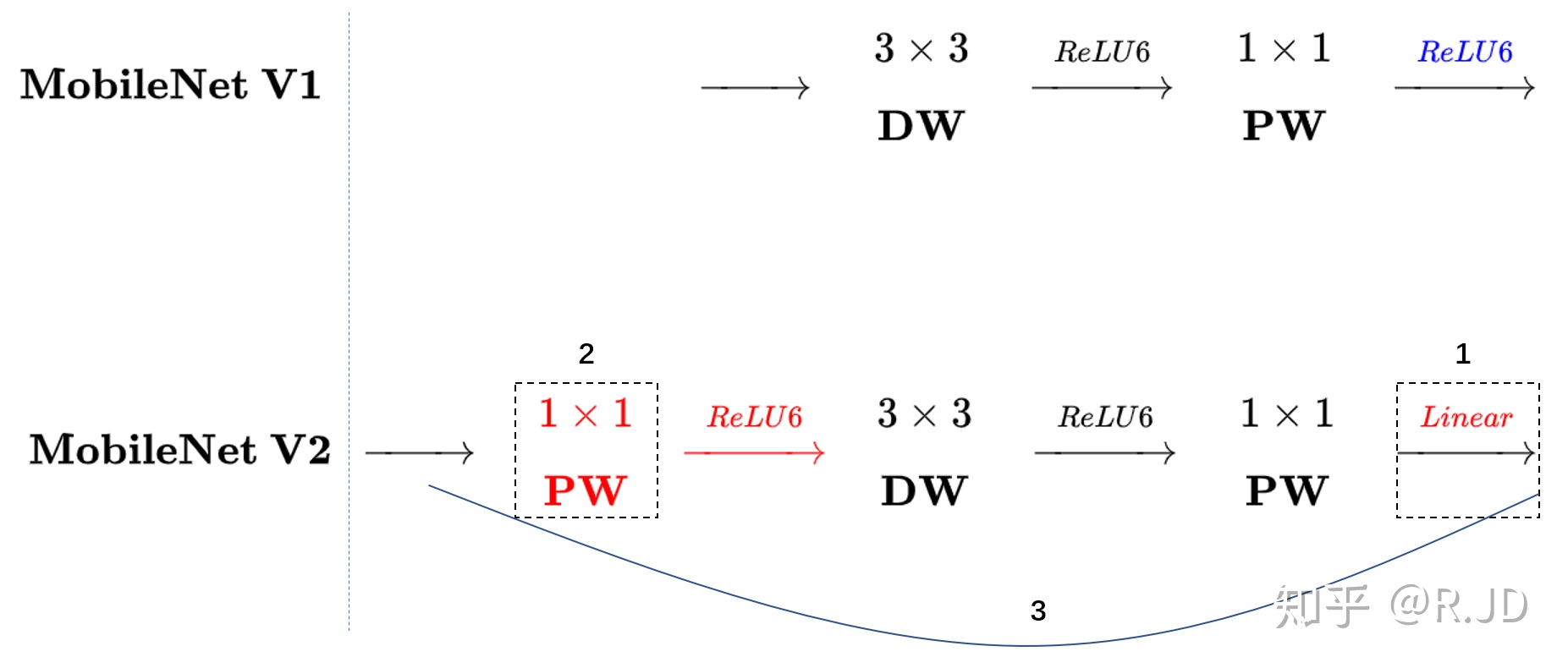
左边是v1的block,没有Shortcut并且带最后的ReLU6。
右边是v2的加入了1×1升维,引入Shortcut并且去掉了最后的ReLU,改为Linear。步长为1时,先进行1×1卷积升维,再进行深度卷积提取特征,再通过Linear的逐点卷积降维。将input与output相加,形成残差结构。步长为2时,因为input与output的尺寸不符,因此不添加shortcut结构,其余均一致。
代码练习
Block
class Block(nn.Module):
    def __init__(self, in_planes, out_planes, expansion, stride):
        super(Block, self).__init__()
        self.stride = stride
        planes = expansion * in_planes
        self.conv1 = nn.Conv2d(in_planes, planes, kernel_size=1, stride=1, padding=0, bias=False)
        self.bn1 = nn.BatchNorm2d(planes)
        self.conv2 = nn.Conv2d(planes, planes, kernel_size=3, stride=stride, padding=1, groups=planes, bias=False)
        self.bn2 = nn.BatchNorm2d(planes)
        self.conv3 = nn.Conv2d(planes, out_planes, kernel_size=1, stride=1, padding=0, bias=False)
        self.bn3 = nn.BatchNorm2d(out_planes)

        if stride == 1 and in_planes != out_planes:
            self.shortcut = nn.Sequential(nn.Conv2d(in_planes, out_planes, kernel_size=1, stride=1, padding=0, bias=False), nn.BatchNorm2d(out_planes))
        if stride == 1 and in_planes == out_planes:
            self.shortcut = nn.Sequential()

    def forward(self, x):
        out = F.relu(self.bn1(self.conv1(x)))
        out = F.relu(self.bn2(self.conv2(out)))
        out = self.bn3(self.conv3(out))

        if self.stride == 1:
            return out + self.shortcut(x)
        else:
            return out
创建MobileNetV2
class MobileNetV2(nn.Module):
    cfg = [(1,  16, 1, 1),
         (6,  24, 2, 1),
         (6,  32, 3, 2),
         (6,  64, 4, 2),
         (6,  96, 3, 1),
         (6, 160, 3, 2),
         (6, 320, 1, 1)]

    def __init__(self, num_classes=10):
        super(MobileNetV2, self).__init__()
        self.conv1 = nn.Conv2d(3, 32, kernel_size=3, stride=1, padding=1, bias=False)
        self.bn1 = nn.BatchNorm2d(32)
        self.layers = self._make_layers(in_planes=32)
        self.conv2 = nn.Conv2d(320, 1280, kernel_size=1, stride=1, padding=0, bias=False)
        self.bn2 = nn.BatchNorm2d(1280)
        self.linear = nn.Linear(1280, num_classes)

    def _make_layers(self, in_planes):
        layers = []
        for expansion, out_planes, num_blocks, stride in self.cfg:
            strides = [stride] + [1]*(num_blocks-1)
            for stride in strides:
                layers.append(Block(in_planes, out_planes, expansion, stride))
                in_planes = out_planes
        return nn.Sequential(*layers)

    def forward(self, x):
        out = F.relu(self.bn1(self.conv1(x)))
        out = self.layers(out)
        out = F.relu(self.bn2(self.conv2(out)))
        out = F.avg_pool2d(out, 4)
        out = out.view(out.size(0), -1)
        out = self.linear(out)
        return out
创建DataLoader
device = torch.device("cuda:0" if torch.cuda.is_available() else "cpu")

transform_train = transforms.Compose([
    transforms.RandomCrop(32, padding=4),
    transforms.RandomHorizontalFlip(),
    transforms.ToTensor(),
    transforms.Normalize((0.4914, 0.4822, 0.4465), (0.2023, 0.1994, 0.2010))])

transform_test = transforms.Compose([
    transforms.ToTensor(),
    transforms.Normalize((0.4914, 0.4822, 0.4465), (0.2023, 0.1994, 0.2010))])

trainset = torchvision.datasets.CIFAR10(root='./data', train=True,  download=True, transform=transform_train)
testset  = torchvision.datasets.CIFAR10(root='./data', train=False, download=True, transform=transform_test)

trainloader = torch.utils.data.DataLoader(trainset, batch_size=128, shuffle=True, num_workers=2)
testloader = torch.utils.data.DataLoader(testset, batch_size=128, shuffle=False, num_workers=2)
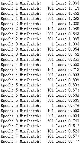
训练模型
for epoch in range(10):
    for i, (inputs, labels) in enumerate(trainloader):
        inputs = inputs.to(device)
        labels = labels.to(device)

        optimizer.zero_grad()

        outputs = net(inputs)
        loss = criterion(outputs, labels)
        loss.backward()
        optimizer.step()

        if i % 100 == 0:
            print('Epoch: %d Minibatch: %5d loss: %.3f' %(epoch + 1, i + 1, loss.item()))

print('Finished Training')
测试
correct = 0
total = 0

for data in testloader:
    images, labels = data
    images, labels = images.to(device), labels.to(device)
    outputs = net(images)
    _, predicted = torch.max(outputs.data, 1)
    total += labels.size(0)
    correct += (predicted == labels).sum().item()

print('Accuracy of the network on the 10000 test images: %.2f %%' % (
    100 * correct / total))

HybridSN
本文主要介绍了采用2D卷积与3D卷积结合的方法来处理高光谱图像,单纯使用2D卷积无法从光谱维数中提取出良好的鉴别特征图,而单纯使用3D卷积计算又太过复杂,所以本文将两者进行结合,提出了HybridSN
网络结构
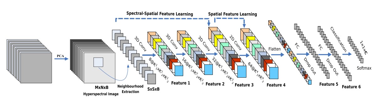
该网络先对输入数据进行PCA操作,使其由
变为
然后将HSI数据立方体划分为重叠的小三维块,再进行三次3D卷积和一次2D卷积,在卷积之后使用flatten和全连接以及dropout操作。
代码练习
构建HybirdSN网络
class HybridSN(nn.Module):
    def __init__(self):
        super(HybridSN, self).__init__()
        self.conv1 = nn.Sequential(
            nn.Conv3d(1, 8, kernel_size=(7,3,3), stride=1, padding=0),
            nn.ReLU(inplace=True)
        )
        self.conv2 = nn.Sequential(
            nn.Conv3d(8, 16, kernel_size=(5,3,3), stride=1, padding=0),
            nn.ReLU(inplace=True)
        )
        self.conv3 = nn.Sequential(
            nn.Conv3d(16, 32, kernel_size=(3,3,3), stride=1, padding=0),
            nn.ReLU(inplace=True)
        )
        self.conv4 = nn.Sequential(
            nn.Conv2d(576, 64, kernel_size=(3,3), stride=1, padding=0),
            nn.ReLU(inplace=True)
        )
        self.fc1 = nn.Linear(18496,256)
        self.fc2 = nn.Linear(256,128)
        self.fc3 = nn.Linear(128,16)
        self.dropout = nn.Dropout(p = 0.4)

    def forward(self, x):
        out = self.conv1(x)
        out = self.conv2(out)
        out = self.conv3(out)
        out = out.reshape(out.shape[0], -1, 19, 19)
        out = self.conv4(out)
        out = out.reshape(out.shape[0], -1)
        out = F.relu(self.dropout(self.fc1(out)))
        out = F.relu(self.dropout(self.fc2(out)))
        out = self.fc3(out)
        return out
创建数据集
def applyPCA(X, numComponents):
    newX = np.reshape(X, (-1, X.shape[2]))
    pca = PCA(n_components=numComponents, whiten=True)
    newX = pca.fit_transform(newX)
    newX = np.reshape(newX, (X.shape[0], X.shape[1], numComponents))
    return newX

def padWithZeros(X, margin=2):
    newX = np.zeros((X.shape[0] + 2 * margin, X.shape[1] + 2 * margin, X.shape[2]))
    x_offset = margin
    y_offset = margin
    newX[x_offset: X.shape[0] + x_offset, y_offset: X.shape[1] + y_offset, :] = X
    return newX

def createImageCubes(X, y, windowSize=5, removeZeroLabels = True):
    margin = int((windowSize - 1) / 2)
    zeroPaddedX = padWithZeros(X, margin=margin)
    patchesData = np.zeros((X.shape[0] * X.shape[1], windowSize, windowSize, X.shape[2]))
    patchesLabels = np.zeros((X.shape[0] * X.shape[1]))
    patchIndex = 0
    for r in range(margin, zeroPaddedX.shape[0] - margin):
        for c in range(margin, zeroPaddedX.shape[1] - margin):
            patch = zeroPaddedX[r - margin:r + margin + 1, c - margin:c + margin + 1]
            patchesData[patchIndex, :, :, :] = patch
            patchesLabels[patchIndex] = y[r-margin, c-margin]
            patchIndex = patchIndex + 1
    if removeZeroLabels:
        patchesData = patchesData[patchesLabels>0,:,:,:]
        patchesLabels = patchesLabels[patchesLabels>0]
        patchesLabels -= 1
    return patchesData, patchesLabels

def splitTrainTestSet(X, y, testRatio, randomState=345):
    X_train, X_test, y_train, y_test = train_test_split(X, y, test_size=testRatio, random_state=randomState, stratify=y)
    return X_train, X_test, y_train, y_test

class_num = 16
X = sio.loadmat('Indian_pines_corrected.mat')['indian_pines_corrected']
y = sio.loadmat('Indian_pines_gt.mat')['indian_pines_gt']

test_ratio = 0.90
patch_size = 25
pca_components = 30

print('Hyperspectral data shape: ', X.shape)
print('Label shape: ', y.shape)

print('\n... ... PCA tranformation ... ...')
X_pca = applyPCA(X, numComponents=pca_components)
print('Data shape after PCA: ', X_pca.shape)

print('\n... ... create data cubes ... ...')
X_pca, y = createImageCubes(X_pca, y, windowSize=patch_size)
print('Data cube X shape: ', X_pca.shape)
print('Data cube y shape: ', y.shape)

print('\n... ... create train & test data ... ...')
Xtrain, Xtest, ytrain, ytest = splitTrainTestSet(X_pca, y, test_ratio)
print('Xtrain shape: ', Xtrain.shape)
print('Xtest  shape: ', Xtest.shape)

Xtrain = Xtrain.reshape(-1, patch_size, patch_size, pca_components, 1)
Xtest  = Xtest.reshape(-1, patch_size, patch_size, pca_components, 1)
print('before transpose: Xtrain shape: ', Xtrain.shape)
print('before transpose: Xtest  shape: ', Xtest.shape)

Xtrain = Xtrain.transpose(0, 4, 3, 1, 2)
Xtest  = Xtest.transpose(0, 4, 3, 1, 2)
print('after transpose: Xtrain shape: ', Xtrain.shape)
print('after transpose: Xtest  shape: ', Xtest.shape)


class TrainDS(torch.utils.data.Dataset):
    def __init__(self):
        self.len = Xtrain.shape[0]
        self.x_data = torch.FloatTensor(Xtrain)
        self.y_data = torch.LongTensor(ytrain)
    def __getitem__(self, index):
        return self.x_data[index], self.y_data[index]
    def __len__(self):
        return self.len

class TestDS(torch.utils.data.Dataset):
    def __init__(self):
        self.len = Xtest.shape[0]
        self.x_data = torch.FloatTensor(Xtest)
        self.y_data = torch.LongTensor(ytest)
    def __getitem__(self, index):
        return self.x_data[index], self.y_data[index]
    def __len__(self):
        return self.len

trainset = TrainDS()
testset  = TestDS()
train_loader = torch.utils.data.DataLoader(dataset=trainset, batch_size=128, shuffle=True, num_workers=2)
test_loader  = torch.utils.data.DataLoader(dataset=testset,  batch_size=128, shuffle=False, num_workers=2)
开始训练
device = torch.device("cuda:0" if torch.cuda.is_available() else "cpu")

net = HybridSN().to(device)
criterion = nn.CrossEntropyLoss()
optimizer = optim.Adam(net.parameters(), lr=0.001)

total_loss = 0
for epoch in range(100):
    for i, (inputs, labels) in enumerate(train_loader):
        inputs = inputs.to(device)
        labels = labels.to(device)
        optimizer.zero_grad()
        outputs = net(inputs)
        loss = criterion(outputs, labels)
        loss.backward()
        optimizer.step()
        total_loss += loss.item()
    print('[Epoch: %d]   [loss avg: %.4f]   [current loss: %.4f]' %(epoch + 1, total_loss/(epoch+1), loss.item()))

print('Finished Training')

测试
count = 0
for inputs, _ in test_loader:
inputs = inputs.to(device)
outputs = net(inputs)
outputs = np.argmax(outputs.detach().cpu().numpy(), axis=1)
if count == 0:
y_pred_test = outputs
count = 1
else:
y_pred_test = np.concatenate( (y_pred_test, outputs) )
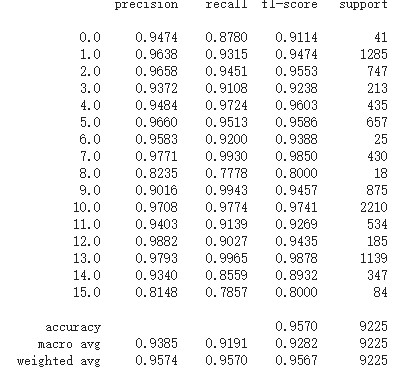
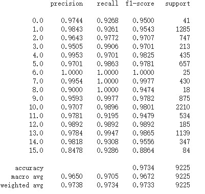
classification = classification_report(ytest, y_pred_test, digits=4)
print(classification)
问题
每次测试的结果都会有一定幅度的变动。

经过百度发现,是由于采用了dropout的原因。在训练代码前加入net.train(),测试代码前加入net.eval(),测试结果就不再变动了。
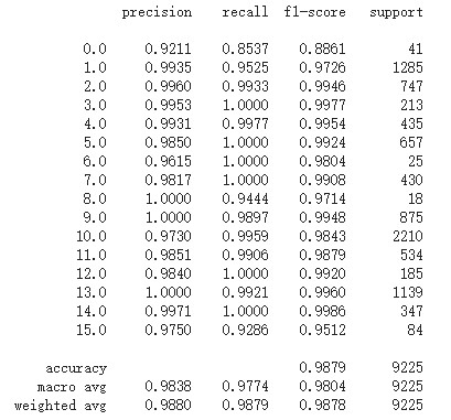
可改进的地方
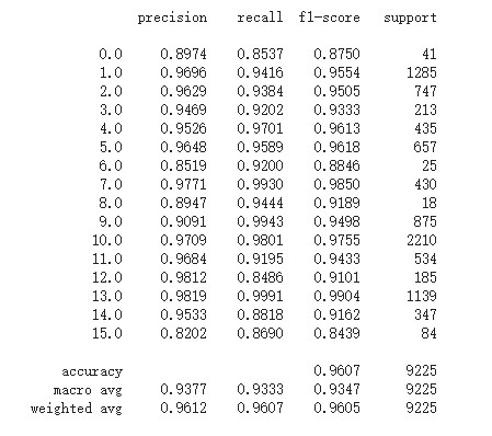
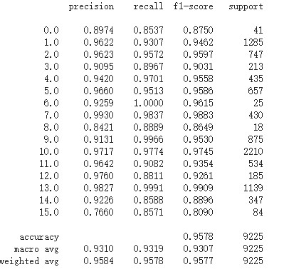
尝试在网络中加入BN,修改后的代码如下:
class HybridSN(nn.Module):
    def __init__(self):
        super(HybridSN, self).__init__()
        self.conv1 = nn.Sequential(
            nn.Conv3d(1, 8, kernel_size=(7,3,3), stride=1, padding=0),
            nn.BatchNorm3d(8),
            nn.ReLU(inplace=True)
        )
        self.conv2 = nn.Sequential(
            nn.Conv3d(8, 16, kernel_size=(5,3,3), stride=1, padding=0),
            nn.BatchNorm3d(16),
            nn.ReLU(inplace=True)
        )
        self.conv3 = nn.Sequential(
            nn.Conv3d(16, 32, kernel_size=(3,3,3), stride=1, padding=0),
            nn.BatchNorm3d(32),
            nn.ReLU(inplace=True)
        )
        self.conv4 = nn.Sequential(
            nn.Conv2d(576, 64, kernel_size=(3,3), stride=1, padding=0),
            nn.BatchNorm2d(64),
            nn.ReLU(inplace=True)
        )
        self.fc1 = nn.Linear(18496,256)
        self.fc2 = nn.Linear(256,128)
        self.fc3 = nn.Linear(128,16)
        self.dropout = nn.Dropout(p = 0.4)

    def forward(self, x):
        out = self.conv1(x)
        out = self.conv2(out)
        out = self.conv3(out)
        out = out.reshape(out.shape[0], -1, 19, 19)
        out = self.conv4(out)
        out = out.reshape(out.shape[0], -1)
        out = F.relu(self.dropout(self.fc1(out)))
        out = F.relu(self.dropout(self.fc2(out)))
        out = self.fc3(out)
        return out
测试发现有2%的提升

 浙公网安备 33010602011771号