Himawari-8 HSD数据解析及辐射定标

1. HSD数据结构介绍

## Full-disk
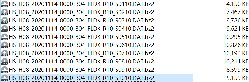
 HS_H08_YYYYMMDD_hhmm_Bbb_FLDK_Rjj_Skkll.DAT

 where YYYY: 4-digit year of observation start time (timeline);
       MM: 2-digit month of timeline;
       DD: 2-digit day of timeline;
       hh: 2-digit hour of timeline;
       mm: 2-gidit minutes of timeline;
       bb: 2-digit band number (varies from "01" to "16");
       jj: spatial resolution ("05": 0.5km, "10": 1.0km, "20": 2.0km);
       kk: segment number (varies from "01" to "10"); and
       ll: total number of segments (fixed to "10").

 example: HS_H08_20150728_2200_B01_FLDK_R10_S0110.DAT

具体命名格式如上，其中需要注意的是kk代表segment number，一开始笔者不明其意，下载了单景分辨率1km的全圆盘影像，发现行列号为(1100*11000)，于是很纳闷为啥圆盘是这么个长方形。思索了很长时间没有结果，于是休息了一会，今天突然发现了原因：segement number编号为01-10，其实是将(11000 * 11000)的圆盘图像分割成了10个小图像!!!

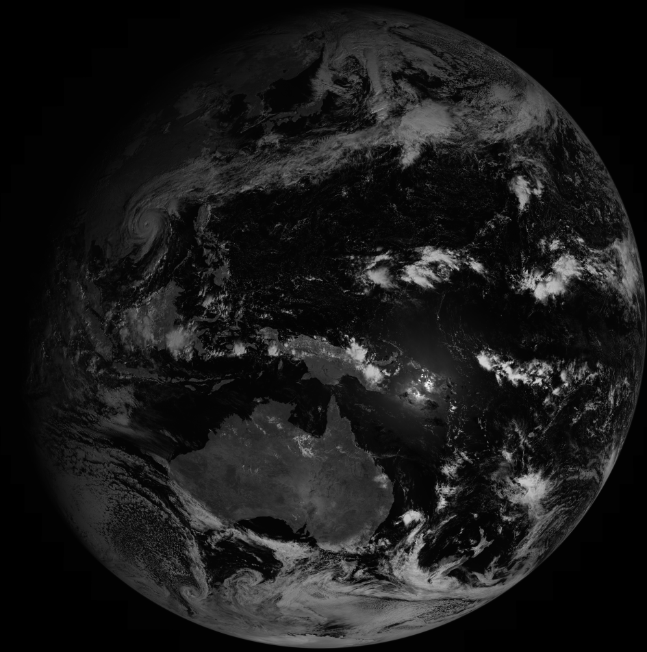
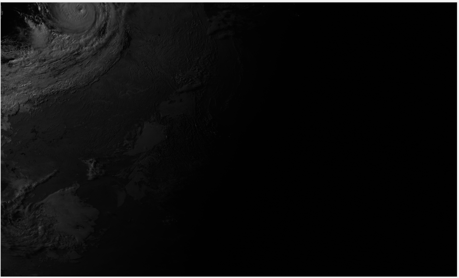
于是立刻编写代码验证想法，一经测试果真如此，下图为数据合成后的结果。

2. DAT文件的读取

了解了Himawari-8 hsd数据的格式后，就可以开始读取每个DAT文件了。下面这个链接给出了DAT文件的数据格式及其python读取方法，其中将DAT文件按一定format读取，转换成了可以打开的txt。

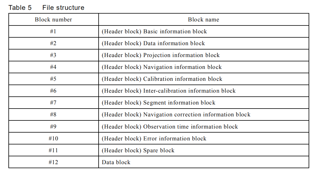
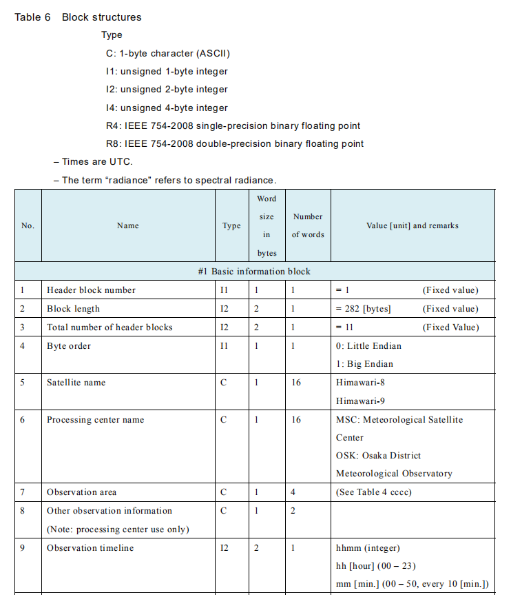
DAT数据由12个block组成，每个block有自己的组织形式，如下图。

https://blog.csdn.net/qq_33339770/article/details/102708243?utm_medium=distribute.pc_relevant.none-task-blog-searchFromBaidu-4.control&depth_1-utm_source=distribute.pc_relevant.none-task-blog-searchFromBaidu-4.control

读取方法如下：1. 对于数据量小的数据可以用f.read()逐字读取

					   2. 对于数据量大的数据用`np.fromfile()`配合**format**读取
					   3. 其实不用`f.seek()`也可以用`re`匹配
					   4. `pandas.read_table()`也可以读取.dat
					   5. **辐射定标**：可在DAT文件中读取定标系数，进行辐射定标；此外**Albedo/Tbb的反射率定标方法有所不同**。

def read_hsd(inputfile):
    '''
    @desc: 打开单个segment图幅，读取.DAT文件中的信息(data/gains/bias...)
    @method: np.fromfile()
    '''
    resolution = int(inputfile[-12:-10])
    if resolution == 10:
        rows = 1100
        cols = 11000
    elif resolution == 20:
        rows = 550
        cols = 5500
    else:
        rows = 2200
        cols = 22000
    # 打开文件
    f = open(inputfile, 'rb')
    # 获取Observation start time
    f.seek(46)
    imgtime = struct.unpack('d', f.read(8))[0]
    # 获取Total header length
    f.seek(70)
    header_length = struct.unpack('i', f.read(4))[0]
    # 获取影像
    formation = [('header', 'S1', header_length), ('pixel', 'i2', rows*cols)]
    imgdata = np.fromfile(inputfile, dtype=formation)['pixel'].reshape(rows, cols)

    '''
    @desc: 下面是辐射定标部分，如果不需要可省略
    '''
    # if resolution != 20:
    #     # 重采样至550行，5500列，可省略
    #     imgdata = imgdata.reshape(550, int(20/resolution), 5500, int(20/resolution)).mean(axis=(1, 3))
    
    # 获取Sun's position
    f.seek(510)
    sun_pos1 = struct.unpack('d', f.read(8))[0]
    # print(sun_pos1)
    f.seek(510+8)
    sun_pos2 = struct.unpack('d', f.read(8))[0]
    # print(sun_pos2)
    f.seek(510+8+8)
    sun_pos3 = struct.unpack('d', f.read(8))[0]
    # print(sun_pos3)
    # 获取Band number
    f.seek(601)
    band_num = int.from_bytes(f.read(2), byteorder='little', signed=False)
    # 获取Gain
    f.seek(617)
    Gain = struct.unpack('d', f.read(8))[0]
    # print(Gain)
    # 获取Offset
    f.seek(625)
    Offset = struct.unpack('d', f.read(8))[0]
    # print(Offset)
    # 计算radiance
    radiance = imgdata*Gain + Offset

    # print(radiance[0][1580])
    # 对前6波段定标成反射率
    if band_num <= 6:
        # 获取radiance to albedo
        f.seek(633)
        cc = struct.unpack('d', f.read(8))[0]
        f.close
        # 计算反射率
        albedo = radiance * cc
        outdata = albedo
    # 后面的波段定标成计算亮温
    else:
        # 获取Central wave length
        f.seek(603)
        wv = struct.unpack('d', f.read(8))[0]
        # 获取radiance to brightness temperature(c0)
        f.seek(633)
        c0 = struct.unpack('d', f.read(8))[0]
        # 获取radiance to brightness temperature(c1)
        f.seek(641)
        c1 = struct.unpack('d', f.read(8))[0]
        # 获取radiance to brightness temperature(c2)
        f.seek(649)
        c2 = struct.unpack('d', f.read(8))[0]
        # 获取Speed of light(c)
        f.seek(681)
        c = struct.unpack('d', f.read(8))[0]
        # 获取Planck constant(h)
        f.seek(689)
        h = struct.unpack('d', f.read(8))[0]
        # 获取Boltzmann constant(k)
        f.seek(697)
        k = struct.unpack('d', f.read(8))[0]
        f.close
        # 计算亮温
        wv = wv * 1e-6
        rad = radiance * 1e6
        Te = h*c/k/wv/(np.log(2*h*c*c/((wv**5)*rad)+1))
        BT = c0 + c1 * Te + c2 * Te * Te
        # 返回值
        outdata = BT

    # 返回：albedo / BT, 时间, 太阳坐标
    sunpos = [sun_pos1, sun_pos2, sun_pos3]
    out = {'pixels': list(outdata.flatten()), 'time': imgtime, 'sun_pos': sunpos}
    return out

3. 经纬度和行列号互转

与FY-4A类似，Full-disk数据在几何校正的时候都需要进行经纬度与行列号的转换，从而把NOM投影转换成等经纬度投影。两者计算的唯一差别在于卫星星下点经纬度、行偏移、列偏移的不同(COFF/LFAC...)，其他公式都一样。

下面给出经纬度与行列号的转换代码：

def calParameter(resolution):
    '''
    @desc: 计算Himawari-8 COFF/CFAC/LOFF/LFAC
    @resolution: 10:1km/20:2km
    '''
    if resolution == 20:
        row = 550
        col = 5500
        COFF = LOFF = 2750.5
        CFAC = LFAC = 20466275
    elif resolution == 10:
        row = 1100
        col = 11000
        COFF = LOFF = 5500.5
        CFAC = LFAC = 40932549
    return COFF, LOFF, CFAC, LFAC

def latlon2linecolumn(lat, lon, resolution):
    """
    经纬度转行列
    (lat, lon) → (line, column)
    resolution：文件名中的分辨率
    line, column
    """
    COFF, LOFF, CFAC, LFAC = calParameter(resolution)
    ea = 6378.137  # 地球的半长轴[km]
    eb = 6356.7523  # 地球的短半轴[km]
    h = 42164  # 地心到卫星质心的距离[km]
    λD = np.deg2rad(140.7)  # 卫星星下点所在经度
    # Step1.检查地理经纬度
    # Step2.将地理经纬度的角度表示转化为弧度表示
    lat = np.deg2rad(lat)
    lon = np.deg2rad(lon)
    # Step3.将地理经纬度转化成地心经纬度
    eb2_ea2 = eb ** 2 / ea ** 2
    λe = lon
    φe = np.arctan(eb2_ea2 * np.tan(lat))
    # Step4.求Re
    cosφe = np.cos(φe)
    re = eb / np.sqrt(1 - (1 - eb2_ea2) * cosφe ** 2)
    # Step5.求r1,r2,r3
    λe_λD = λe - λD
    r1 = h - re * cosφe * np.cos(λe_λD)
    r2 = -re * cosφe * np.sin(λe_λD)
    r3 = re * np.sin(φe)
    # Step6.求rn,x,y
    rn = np.sqrt(r1 ** 2 + r2 ** 2 + r3 ** 2)
    x = np.rad2deg(np.arctan(-r2 / r1))
    y = np.rad2deg(np.arcsin(-r3 / rn))
    # Step7.求c,l
    column = COFF + x * 2 ** -16 * CFAC
    line = LOFF + y * 2 ** -16 * LFAC
    return np.rint(line).astype(np.uint16), np.rint(column).astype(np.uint16)

4. 几何校正

最后就是进行几何校正了，需要我们设定目标区的经纬度范围（如Lon: 90-120 Lat: 30-50），然后根据pixelSize计算出geotrans、col/row等信息。最后根据经纬度反算出行列号，进而求得行列号对应的像元的值，写入数组，这样就完成了几何校正。

切记行列号顺序不可弄错，numpy先行后列，gdal先列后行。

def hsd2tif(arr, lonMin, lonMax, latMin, latMax, pixelSize, file_out):
    '''
    @desc: 几何校正，输出tif
    '''
    col = np.ceil(lonMax-lonMin)/pixelSize
    row = np.ceil(latMax-latMin)/pixelSize
    col = int(col)
    row = int(row)
    xnew = np.linspace(latMin, latMax, row)
    ynew = np.linspace(lonMin, lonMax, col)
    xnew, ynew = np.meshgrid(xnew, ynew)
    dataGrid = np.zeros((row, col))  # numpy数组先行后列!!!
    
    index = {}
    for i in tqdm(range(row)):
        for j in tqdm(range(col)):
            lat = xnew[i][j]
            lon = ynew[i][j]
            h8Row = 0
            h8Col = 0
            if index.get((lat, lon)) == None:
                h8Row, h8Col = latlon2linecolumn(lat, lon, 10)
                index[(lat, lon)] = h8Row, h8Col
            else:
                h8Row, h8Col = index.get((lat, lon))
                
            if (0<=h8Row<11000) and (0<=h8Col<11000):
                dataGrid[i][j] = arr[h8Row, h8Col]
                print("Worked!" + str(dataGrid[i][j]))
            else:
                print("该坐标(%s, %s)不在影像中"%(lon, lat))

    geotrans = (lonMin, pixelSize, 0, latMax, 0, -pixelSize)
    srs = osr.SpatialReference()
    srs.ImportFromEPSG(4326)
    proj = srs.ExportToWkt()
    raster2tif(dataGrid, geotrans, proj, file_out)

5. 后记

到这里我们的HSD数据解析和辐射定标就完成了。

后续还可以调用6S模型进行大气校正，这也需要更多的地理信息如(SALA/SAZA/SOLA/SOZA)，https://blog.csdn.net/qq_33339770/article/details/103023725 这里给出了一些参数的计算方法。
根据经纬度反算行列号，计算速度偏慢。

如果需要快速出图的话，建议使用已经计算好的经纬度栅格图进行GLT校正，速度会快很多。（ENVI有GLT校正模块，gdal应该也有，后续可以建立好经纬度栅格图然后调用gdal来批量几何校正）

posted @ 2020-12-15 11:56 Rser_ljw 阅读(3922) 评论(7) 编辑收藏举报

会员力量，点亮园子希望

刷新页面返回顶部

Rser_ljw

亦是书生，亦是侠客

Himawari-8 HSD数据解析及辐射定标

Himawari-8 HSD数据解析及辐射定标

1. HSD数据结构介绍

2. DAT文件的读取

3. 经纬度和行列号互转

4. 几何校正

5. 后记

公告