Hough变换之直线检测

1.Hough Transform 的算法思想

在直角坐标系和极坐标系中，点、线是对偶关系。

即直角坐标系中的点是极坐标系中的线，直角坐标系中的线是极坐标系中的点。反之也成立。

如下图所示，想要检测图像中的直线，可以转化为检测极坐标系中的点(θ,r)。

---

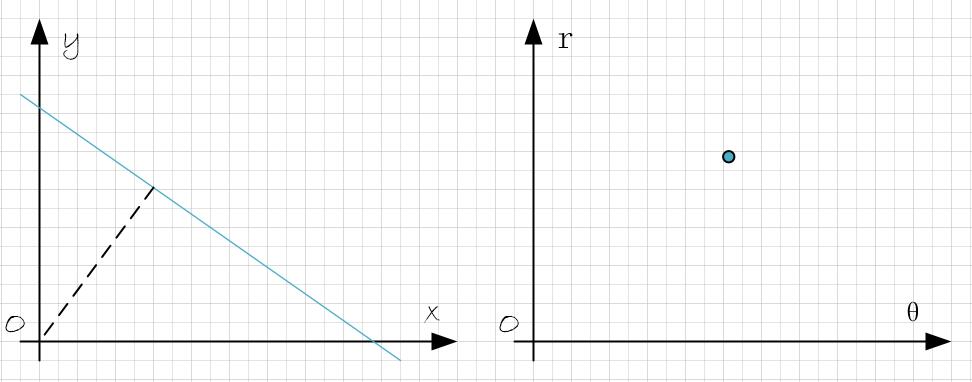
2.Hough空间的表示

如下图所示，图像中直线的表示，由斜率和截距表示，而极坐标中用(θ,r)表示，并且存在下式关系：

r=cos(θ)⋅x+sin(θ)⋅y

对于点(x0,y0)，代入上式，在极坐标中就是一条线（很多对(θ,r)点）:

r=cos(θ)⋅x0+sin(θ)⋅y0

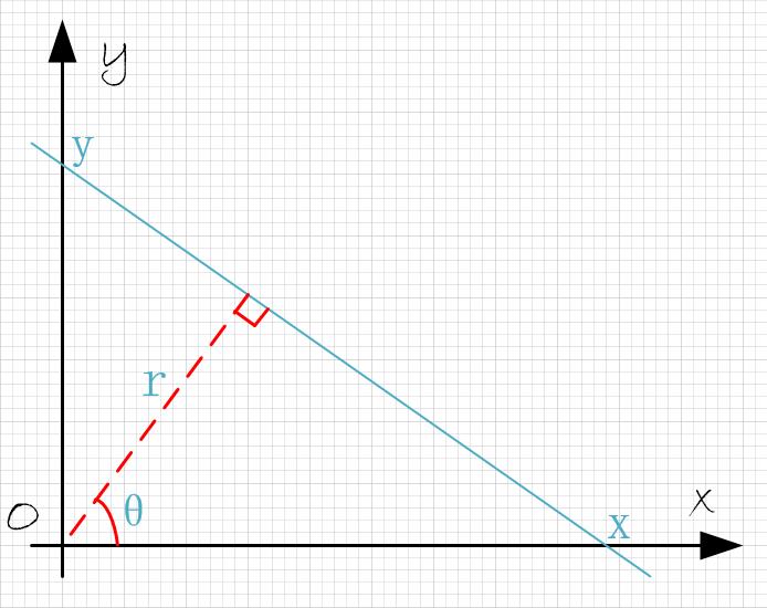
r，θ 就是一对Hough空间的变量表示。

旋转的 θ 不容易表示，若将 r，θ 看成直角坐标空间。一个点(x0,y0), 就是一个正弦曲线。

r=cos(θ)⋅x0+sin(θ)⋅y0

如下图所示，左图直角坐标系中的一个点，对应于右图 r-θ 空间的一条正弦曲线。

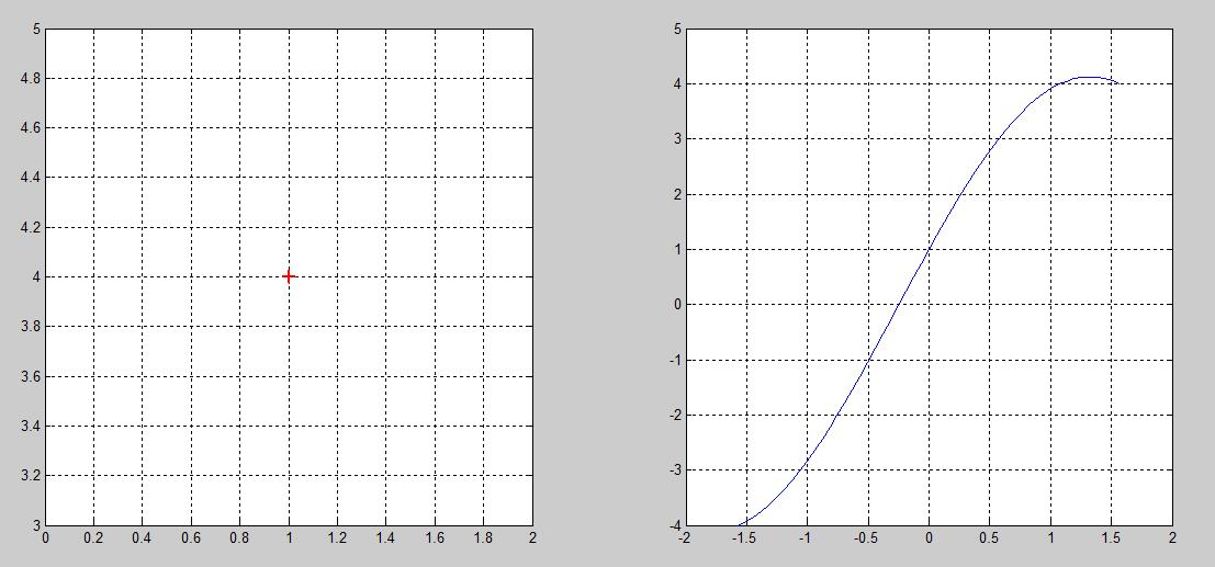
如下图，直角坐标系中的多个点，对应于 r-θ 空间的多条正弦曲线。

直角坐标系的三点共线，对应于 r-θ 空间的多线共点。

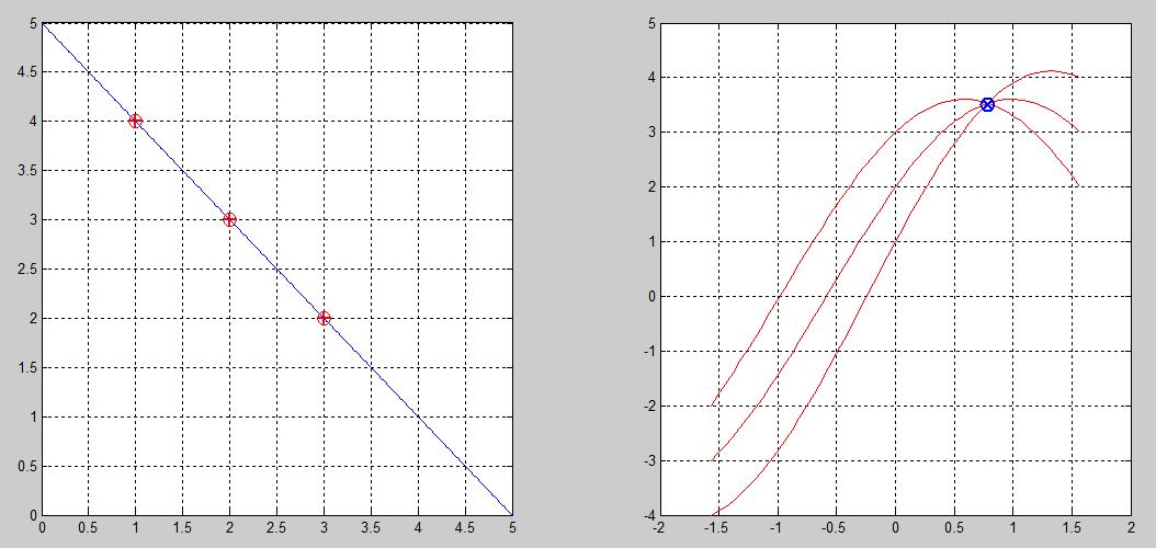
因此，我们可以通过检测 r-θ 空间的交集点，来检测原始空间的线段。

接下来，就是要考虑 将r，θ离散化，形成离散化的Hough空间，类似于一个矩阵/图像(如下图)，用于统计交集点的个数。

---

3.Hough变换代码分析

以下是使用Matlab进行直线检测的代码。

Hough Transform

首先预处理，转为二值图像：

I  = imread('road.jpg');
I = rgb2gray(I);
BW = edge(I,'canny');

然后进行霍夫变换：

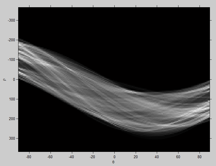
[H,T,R] = hough(BW,'RhoResolution',0.5,'Theta',-90:0.5:89.5);
imshow(H,[],'XData',T,'YData',R,'InitialMagnification','fit');
xlabel('\theta'), ylabel('\rho');
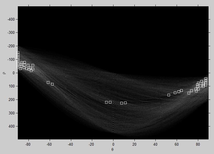
axis on, axis normal, hold on;

检测hough域极值点

P  = houghpeaks(H,50,'threshold',ceil(0.3*max(H(:))));
x = T(P(:,2));
y = R(P(:,1));
plot(x,y,'s','color','white');

检测直线

% Find lines and plot them
lines = houghlines(BW,T,R,P,'FillGap',7,'MinLength',100);
figure, imshow(I), hold on
max_len = 0;
for k = 1:length(lines)
    xy = [lines(k).point1; lines(k).point2];
    plot(xy(:,1),xy(:,2),'LineWidth',2,'Color','green');

    % plot beginnings and ends of lines
    plot(xy(1,1),xy(1,2),'x','LineWidth',2,'Color','yellow');
    plot(xy(2,1),xy(2,2),'x','LineWidth',2,'Color','red');

    % determine the endpoints of the longest line segment
    len = norm(lines(k).point1 - lines(k).point2);
    if ( len > max_len)
        max_len = len;
        xy_long = xy;
    end
end

% highlight the longest line segment
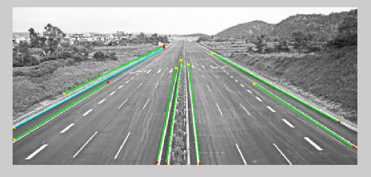
plot(xy_long(:,1),xy_long(:,2),'LineWidth',2,'Color','cyan');

实验结果

r-θ 空间及前50个极值点：

最终车道直线检测结果：

---

[注] 所有的代码可以在此处免费下载：http://download.csdn.net/detail/ws_20100/9492054