Seurat单细胞测序中高变异基因的选择程序验证

数据来源：https://www.jianshu.com/p/4f7aeae81ef1

1、

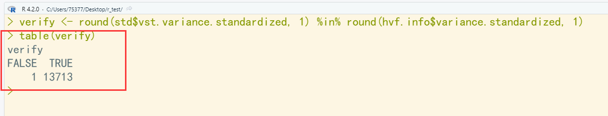
library(dplyr)
library(Seurat)
library(patchwork)
# Load the PBMC dataset
pbmc.data <- Read10X(data.dir = "C:/Users/75377/Desktop/r_test/hg19")
# Initialize the Seurat object with the raw (non-normalized data).
pbmc <- CreateSeuratObject(counts = pbmc.data, project = "pbmc3k", min.cells = 3, min.features = 200)
pbmc
## An object of class Seurat 
## 13714 features across 2700 samples within 1 assay 
## Active assay: RNA (13714 features, 0 variable features)
# The [[ operator can add columns to object metadata. This is a great place to stash QC stats
pbmc[["percent.mt"]] <- PercentageFeatureSet(pbmc, pattern = "^MT-")
# Visualize QC metrics as a violin plot
VlnPlot(pbmc, features = c("nFeature_RNA", "nCount_RNA", "percent.mt"), ncol = 3)
# FeatureScatter is typically used to visualize feature-feature relationships, but can be used
# for anything calculated by the object, i.e. columns in object metadata, PC scores etc.

plot1 <- FeatureScatter(pbmc, feature1 = "nCount_RNA", feature2 = "percent.mt")
plot2 <- FeatureScatter(pbmc, feature1 = "nCount_RNA", feature2 = "nFeature_RNA")
plot1 + plot2

pbmc <- subset(pbmc, subset = nFeature_RNA > 200 & nFeature_RNA < 2500 & percent.mt < 5)

pbmc <- NormalizeData(pbmc)

pbmc <- FindVariableFeatures(pbmc, selection.method = "vst", nfeatures = 2000)

# Identify the 10 most highly variable genes
top10 <- head(VariableFeatures(pbmc), 10)

# plot variable features with and without labels
plot1 <- VariableFeaturePlot(pbmc)
plot2 <- LabelPoints(plot = plot1, points = top10, repel = TRUE)
plot1 + plot2

std <- pbmc[["RNA"]]@meta.features
std <- as.data.frame(std)
fwrite(std, "std.txt", row.names = T, col.names = T, sep = "\t", quote = F)

count <- pbmc[["RNA"]]@counts       ## 原始的counts计数
count <- as.data.frame(count)

mean <- apply(count, 1, mean)            ## 按行求均值
variance <- apply(count, 1, var)         ## 按行求方差
hvf.info <- data.frame(mean, variance)   ## 生成数据框
hvf.info$variance.expected <- 0          ## 添加列并赋值
hvf.info$variance.standardized <- 0
not.const <- hvf.info$variance > 0

fit <- loess(                            ## 根据平均值和方差进行拟合
  formula = log10(x = variance) ~ log10(x = mean),
  data = hvf.info[not.const, ],
  span = 0.3
)
hvf.info$variance.expected[not.const] <- 10 ^ fit$fitted    ## 计算期望方差

count_std <- matrix(nrow = nrow(count), ncol = ncol(count)) ## 生成标准化计数数据框

identical(rownames(count), rownames(hvf.info))

clip_max <- sqrt(ncol(count_std))                           ## 计算修剪的最大值
clip_max
for (i in 1:nrow(count_std)) {
  count_std[i,] <- (as.numeric(count[i,]) -  hvf.info[i,1])/sqrt(hvf.info[i,3])  ## 标准化计数
  count_std[i,][count_std[i,] >=clip_max] <- clip_max         ## 修剪数据
  hvf.info[i,4] <- var(as.numeric(count_std[i,]))                     ## 计算标准化数据后的期望方差
}

head(std)         ## 流程中的标准结果
head(hvf.info)    ## 手动生成的结果
verify <- round(std$vst.variance.standardized, 1) %in% round(hvf.info$variance.standardized, 1) 
table(verify)     ## 统计验证结果，有一个不一致，可能是四舍五入问题

002、改善程序运行效率

dat <- read.table("dat.txt", row.names = 1, header = T)
dim(dat)
dat[1:5, 1:5]

vst.mean <- apply(dat, 1, mean)
vst.variance <- apply(dat, 1, var)

hvf.info <- data.frame(vst.mean, vst.variance)

hvf.info$variance.expected <- 0
hvf.info$variance.standardized <- 0
not.const <- hvf.info$vst.variance > 0
not.const
head(hvf.info)

fit <- loess(
  formula = log10(vst.variance) ~ log10(vst.mean),
  data = hvf.info[not.const, ],
  span = 0.3
)

hvf.info$variance.expected[not.const] <- 10 ^ fit$fitted
head(hvf.info)

max_chip <- sqrt(2638)

head(hvf.info)


a <- hvf.info[,1]
b <- sqrt(hvf.info[,3])

dat <- t(dat)
std_count <- dat

for (i in 1:ncol(dat)) {
  std_count[,i] <- (dat[,i] - a[i])/b[i]
  std_count[,i][std_count[,i] >= max_chip] <- max_chip
  
  hvf.info[i, 4] <- var(std_count[,i])
}

write.table(hvf.info, "xxx.txt", row.names = T, col.names = T, sep = "\t", quote = F)