CNN、RNN、LSTM练习汇总

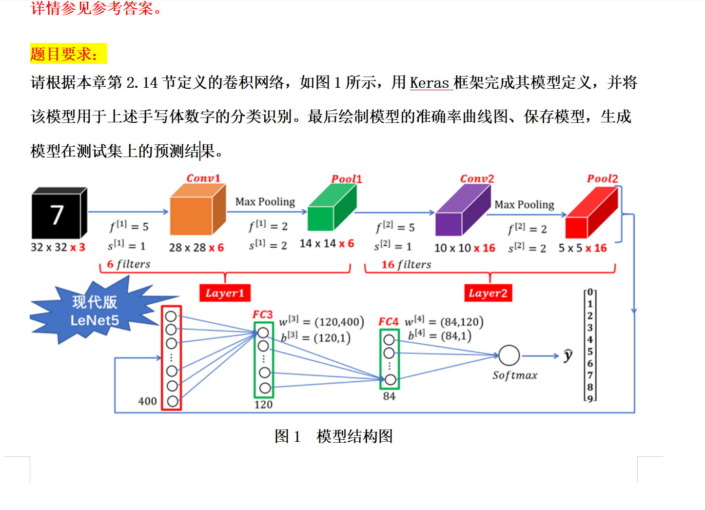
1.手写数字识别

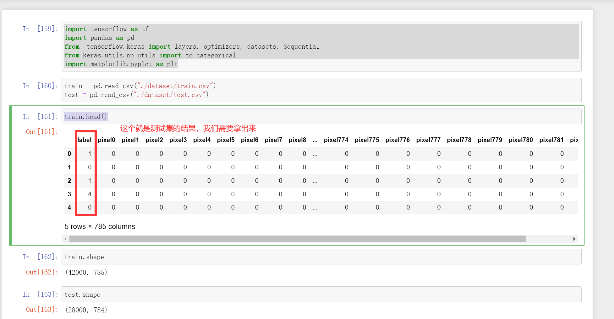
加载数据：

import tensorflow as tf
import pandas as pd
from  tensorflow.keras import layers, optimizers, datasets, Sequential
from keras.utils.np_utils import to_categorical
import matplotlib.pyplot as plt

train = pd.read_csv("./dataset/train.csv")
test = pd.read_csv("./dataset/test.csv")
train.head()
train.shape,test.shape

数据处理

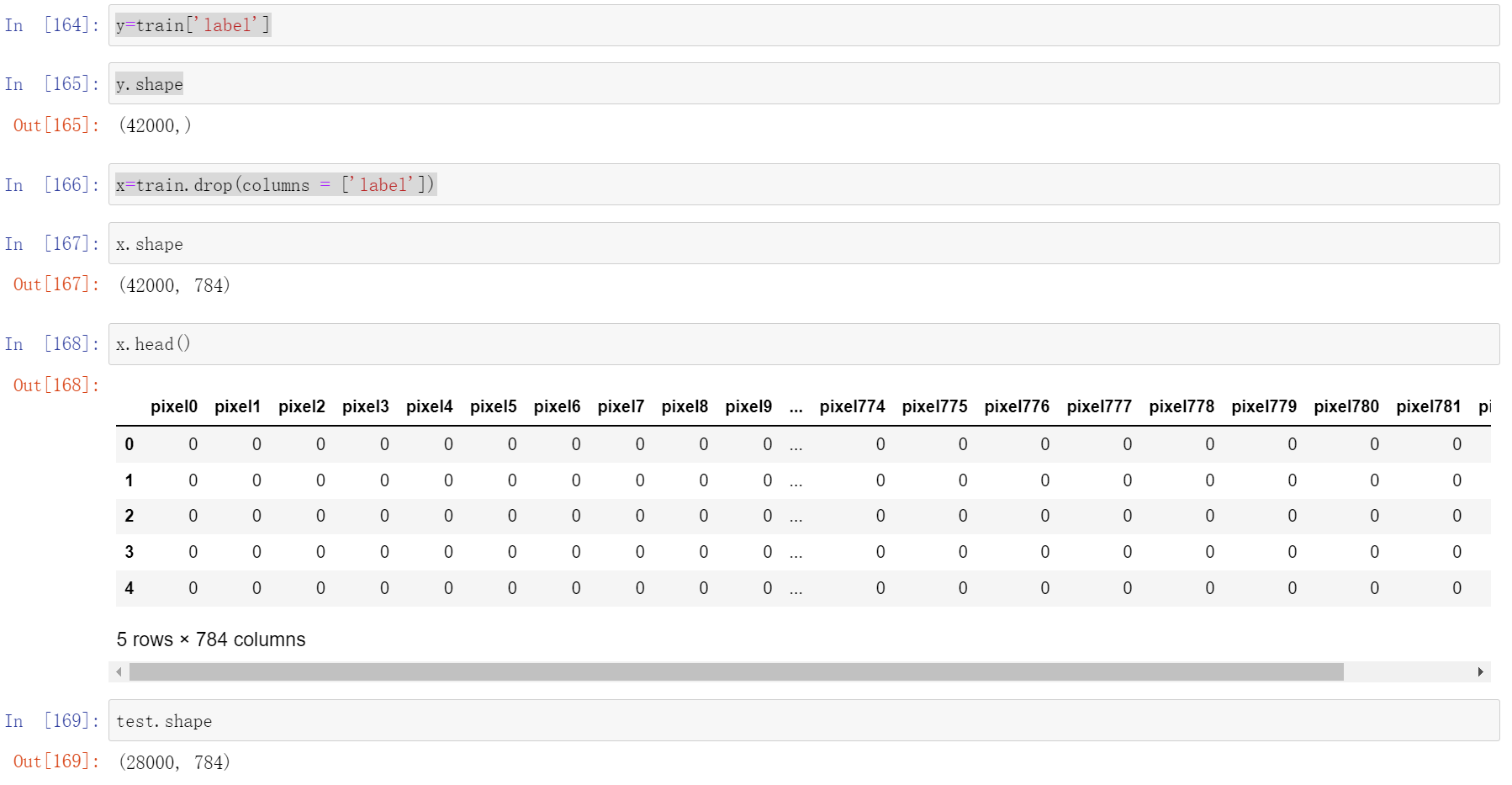
y=train['label']
x=train.drop(columns = ['label'])
y.shape
x.shape

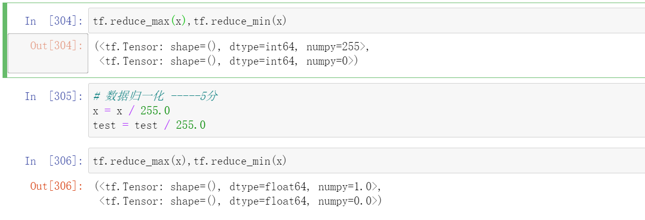
数据归一化

tf.reduce_max(x),tf.reduce_min(x)
# 数据归一化,无量纲化
x = x / 255.0
test = test / 255.0
tf.reduce_max(x),tf.reduce_min(x)

分割数据集

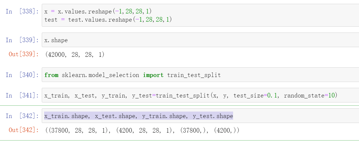
x = x.values.reshape(-1,28,28,1)
test = test.values.reshape(-1,28,28,1)

from sklearn.model_selection import train_test_split
x_train, x_test, y_train, y_test=train_test_split(x, y, test_size=0.1, random_state=10)
x_train.shape, x_test.shape, y_train.shape, y_test.shape

转化成onehot编码
这两种方法都行

#y_train = to_categorical(y_train, num_classes = 10)
#y_test = to_categorical(y_test, num_classes = 10)
y_train=tf.one_hot(y_train, depth=10)
y_test=tf.one_hot(y_test, depth=10)

模型定义

model = Sequential([ # 5 units of conv + max pooling
    # unit 1:
    layers.Conv2D(6, kernel_size=[3, 3], padding="same", activation=tf.nn.relu),
    layers.Conv2D(6, kernel_size=[3, 3], padding="same", activation=tf.nn.relu),
    layers.MaxPool2D(pool_size=[2, 2], strides=2, padding='same'),

    # unit 2
    layers.Conv2D(16, kernel_size=[3, 3], padding="same", activation=tf.nn.relu),
    layers.Conv2D(16, kernel_size=[3, 3], padding="same", activation=tf.nn.relu),
    layers.MaxPool2D(pool_size=[2, 2], strides=2, padding='same'),

    layers.Flatten(),
    layers.Dense(120, activation=tf.nn.relu),
    layers.Dropout(0.25),
    layers.Dense(84, activation=tf.nn.relu),
    layers.Dropout(0.25),
    layers.Dense(10,activation = "softmax"),
	#注意最后一层是"softmax"
])

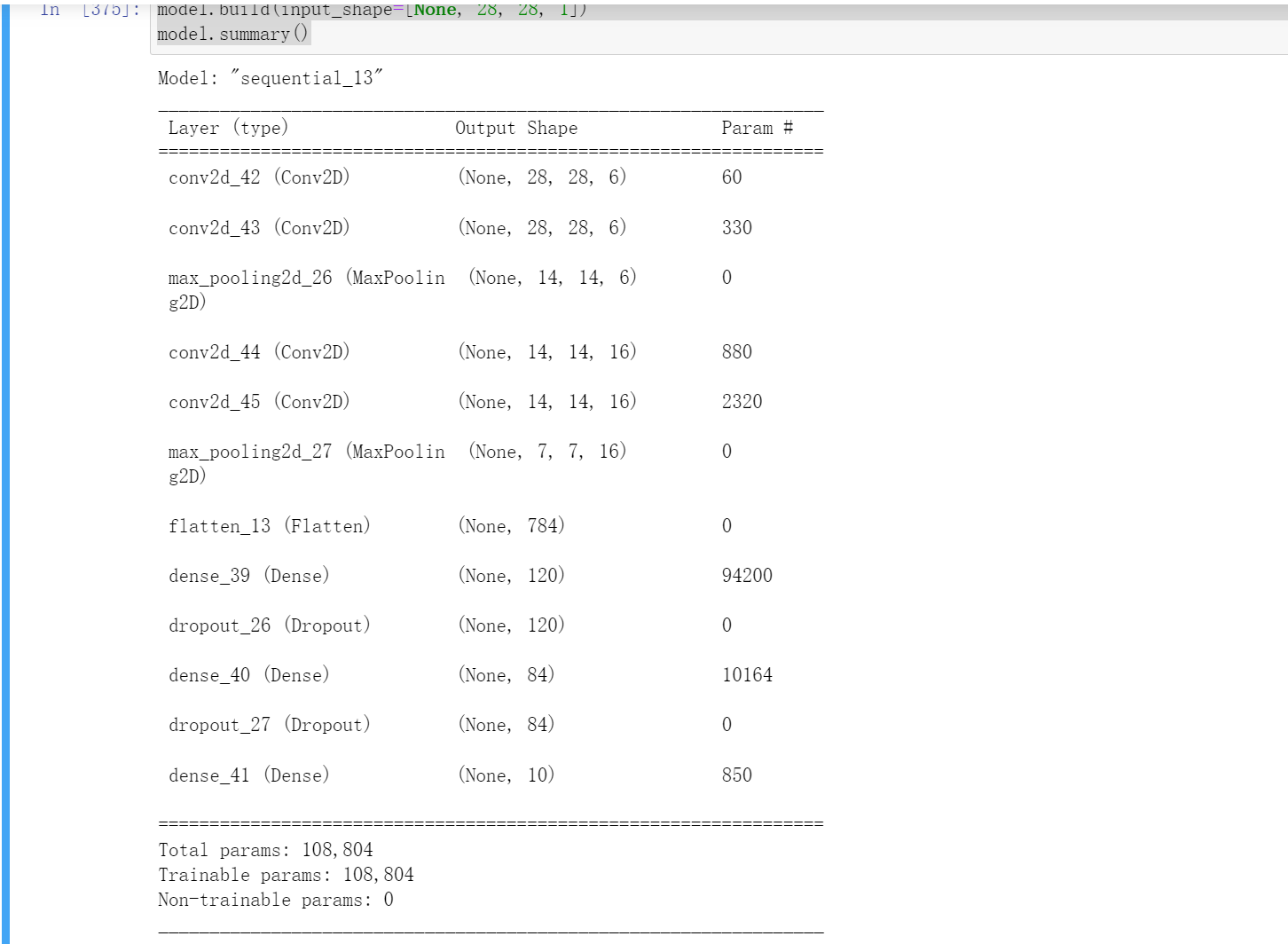
model.build(input_shape=[None, 28, 28, 1])
model.summary()

compile和fit

model.compile(optimizer="Adamax",
                  loss="categorical_crossentropy", metrics=["accuracy"])

optimizer可以选择
SGD#
RMSprop
Adam
Adadelta
Adagrad
Adamax
Nadam
Ftrl
这个具体用法可以看这个中文官网

其中这个loss='categorical_crossentropy'这个是分类交叉熵函数
mean_squared_error：均方误差
categorical_crossentropy：分类交叉熵
binary_crossentropy：二元交叉熵
sparse_categorical_crossentropy：稀疏分类交叉熵
mean_absolute_error：平均绝对误差
hinge：hinge损失函数
squared_hinge：平方hinge损失函数
cosine_proximity：余弦相似度损失函数

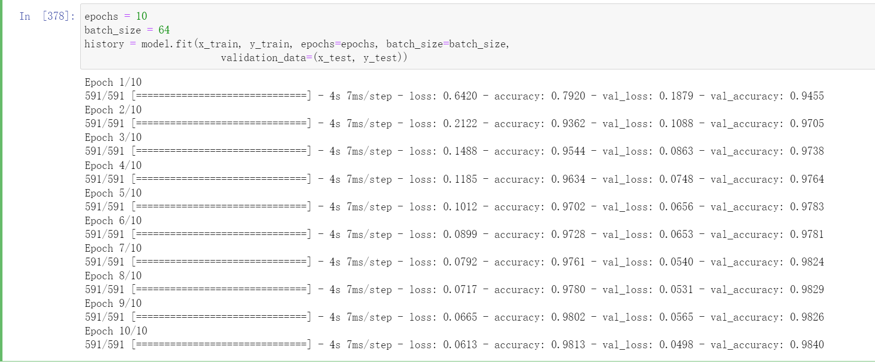
epochs = 10
batch_size = 64
history = model.fit(x_train, y_train, epochs=epochs, batch_size=batch_size,
                        validation_data=(x_test, y_test))

keras中的类History对象有两个属性 history 和 epoch
history.epoch返回一个列表，列表的值是 0 ~ 训练时指定的epoch−1−1
history.history返回一个字典，字典有4个键值key，分别是accuracy、val_accuracy、loss和val_loss，每个key的value均是一个列表，列表的长度=history.epoch的长度=模型训练时指定的epoch数,这些可以用在下面的作图上。
然后这个validation_data中的是验证集特征，和验证集结果

这里我们用到的主要是history.history的4个键值，下面详细介绍
首先我们来介绍一下训练集train和测试集test
训练集是参与网络模型训练的数据集
测试集是对网络模型的性能进行评估的数据集，一般不参与网络模型的训练
验证集是用来用来调整网络超参数的数据集（用的不多）
一般来说整个数据集中训练集和测试集的比例是7：3，有验证集时的比例是6：2：2
accuracy和loss均是描述训练集的
accuracy是每轮训练，训练集的准确度
loss是每轮训练，训练集的损失程度
val_accuracy是每轮训练，验证集的准确度
val_loss是每轮训练，验证集的损失程度
val_accuracy和val_loss均是描述验证集的
但验证集一般不怎么用，一般是用测试集代替验证集，所以才有了训练模型fit函数内的validation_data参数传的是测试集，故这两个对象代表的也可以是测试集

作图

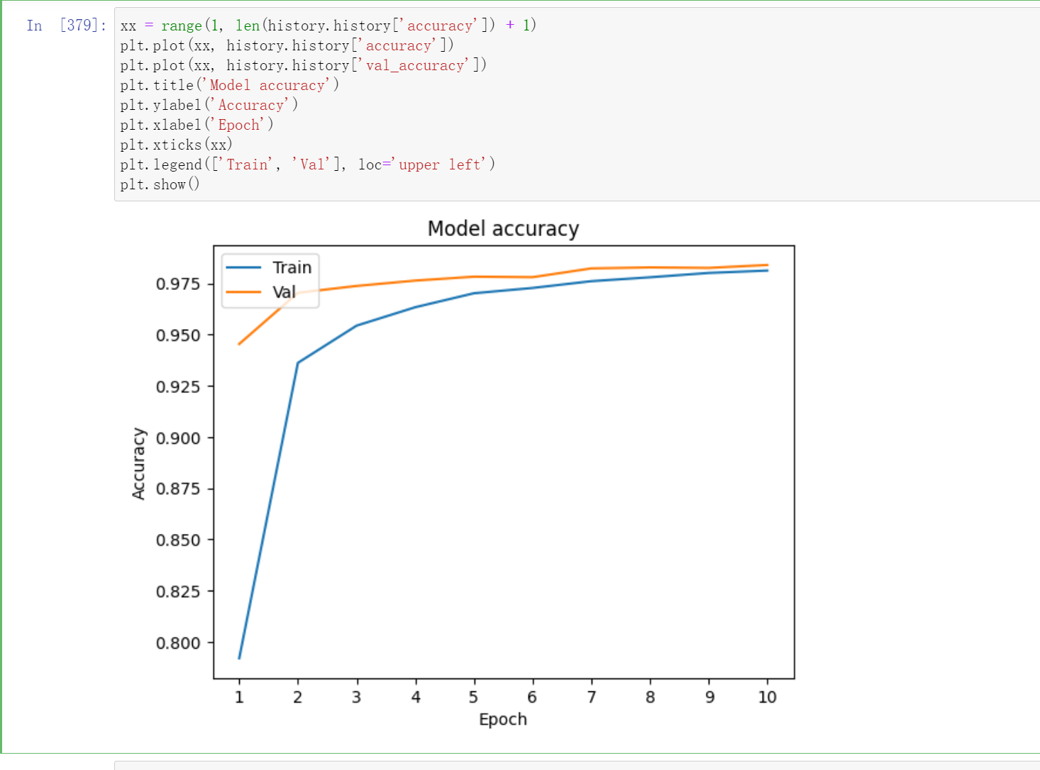
xx = range(1, len(history.history['accuracy']) + 1)
plt.plot(xx, history.history['accuracy'])
plt.plot(xx, history.history['val_accuracy'])
plt.title('Model accuracy')
plt.ylabel('Accuracy')
plt.xlabel('Epoch')
plt.xticks(xx)
plt.legend(['Train', 'Val'], loc='upper left')
plt.show()

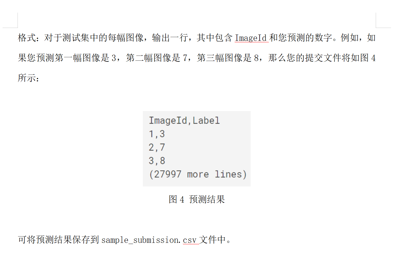
预测结果保存

import numpy as np
#模型预测并保存预测结果到predict_result.csv  ----5分
results = model.predict(test)
results = np.argmax(results,axis = 1)

results = pd.Series(results,name="Label")
submission = pd.concat([pd.Series(range(1,28001),name = "ImageId"),results],axis = 1)

submission.to_csv("predict_result.csv",index=False)

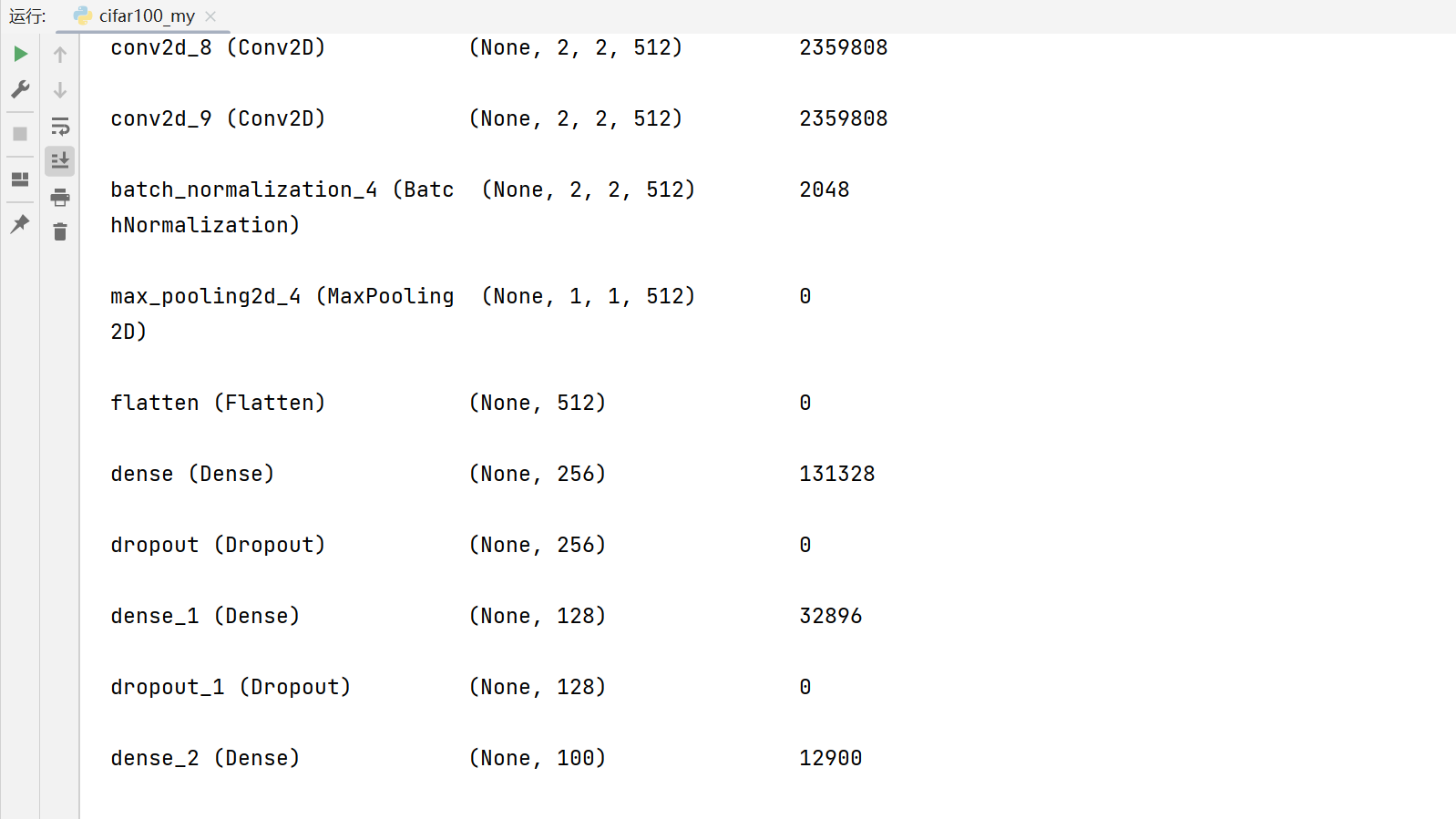
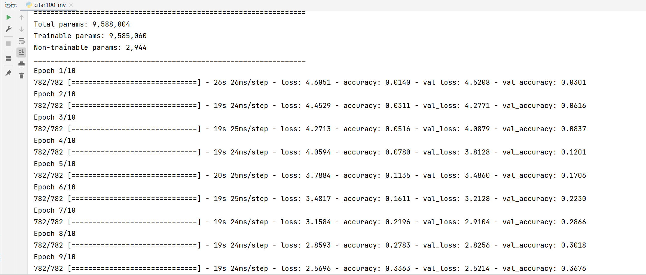
2 cifar100

import  os
os.environ['TF_CPP_MIN_LOG_LEVEL']='2'

import  tensorflow as tf
from    tensorflow.keras import layers, optimizers, datasets, Sequential
from keras.utils.np_utils import to_categorical
import matplotlib.pyplot as plt
tf.random.set_seed(2345)


# 设置采用GPU训练程序
gpus = tf.config.list_physical_devices("GPU")  # 获取电脑GPU列表
if gpus:  # gpus不为空
    gpu0 = gpus[0]  # 选取GPU列表中的第一个
    tf.config.experimental.set_memory_growth(gpu0, True)  # 设置GPU显卡按需使用
    tf.config.set_visible_devices([gpu0], "GPU")  # 设置GPU可见的设备清单，默认是都可见，这里只设置了gpu0可见


model = Sequential([ # 5 units of conv + max pooling
    # unit 1:32
    layers.Conv2D(64, kernel_size=[3, 3], padding="same", activation=tf.nn.relu),
    layers.Conv2D(64, kernel_size=[3, 3], padding="same", activation=tf.nn.relu),
    layers.BatchNormalization(),
    layers.MaxPool2D(pool_size=[2, 2], strides=2, padding='same'),

    # unit 2:16
    layers.Conv2D(128, kernel_size=[3, 3], padding="same", activation=tf.nn.relu),
    layers.Conv2D(128, kernel_size=[3, 3], padding="same", activation=tf.nn.relu),
    layers.BatchNormalization(),
    layers.MaxPool2D(pool_size=[2, 2], strides=2, padding='same'),

    # unit 3:8
    layers.Conv2D(256, kernel_size=[3, 3], padding="same", activation=tf.nn.relu),
    layers.Conv2D(256, kernel_size=[3, 3], padding="same", activation=tf.nn.relu),
    layers.BatchNormalization(),
    layers.MaxPool2D(pool_size=[2, 2], strides=2, padding='same'),

    # unit 4:4
    layers.Conv2D(512, kernel_size=[3, 3], padding="same", activation=tf.nn.relu),
    layers.Conv2D(512, kernel_size=[3, 3], padding="same", activation=tf.nn.relu),
    layers.BatchNormalization(),
    layers.MaxPool2D(pool_size=[2, 2], strides=2, padding='same'),

    # unit 5:2
    layers.Conv2D(512, kernel_size=[3, 3], padding="same", activation=tf.nn.relu),
    layers.Conv2D(512, kernel_size=[3, 3], padding="same", activation=tf.nn.relu),
    layers.BatchNormalization(),
    layers.MaxPool2D(pool_size=[2, 2], strides=2, padding='same'),

    layers.Flatten(),
    layers.Dense(256, activation=tf.nn.relu),
    layers.Dropout(0.5),
    layers.Dense(128, activation=tf.nn.relu),
    layers.Dropout(0.5),
    layers.Dense(100, activation='softmax'),
])



def preprocess(x, y):
    # [0~1]
    x = tf.cast(x, dtype=tf.float32) / 255.
    y = tf.cast(y, dtype=tf.int32)
    return x,y


(x,y), (x_test, y_test) = datasets.cifar100.load_data()


y = tf.squeeze(y, axis=1)
y_test = tf.squeeze(y_test, axis=1)
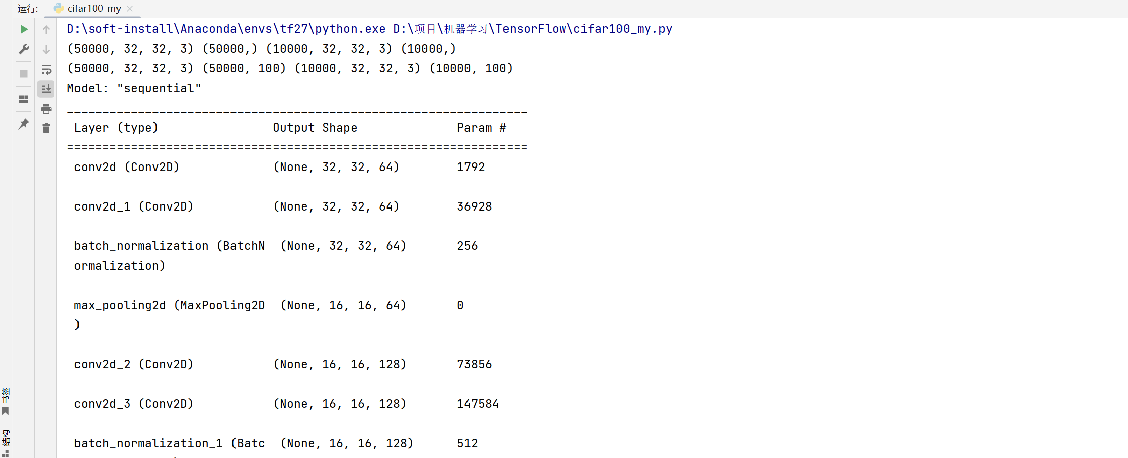
print(x.shape, y.shape, x_test.shape, y_test.shape)

y = to_categorical(y, num_classes = 100)

y_test = to_categorical(y_test, num_classes = 100)

print(x.shape, y.shape, x_test.shape, y_test.shape)


def main():
    # # 这里一定不要忘了
    model.build(input_shape=[None, 32, 32, 3])
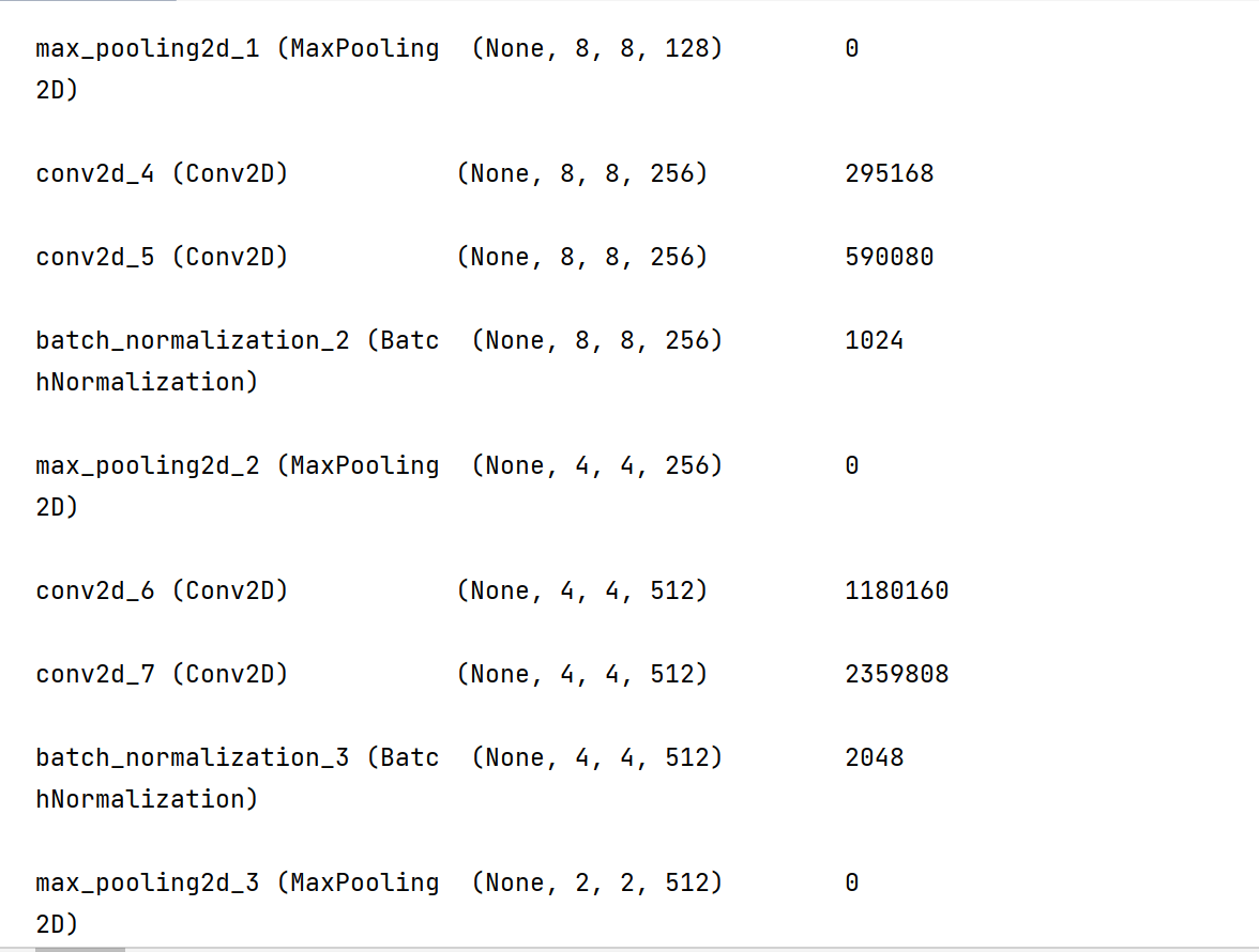
    model.summary()

    model.compile(optimizer="Adamax",
                  loss="categorical_crossentropy", metrics=["accuracy"])

    epochs = 10
    batch_size = 64
    history = model.fit(x, y, epochs=epochs, batch_size=batch_size,
                        validation_data=(x_test, y_test))

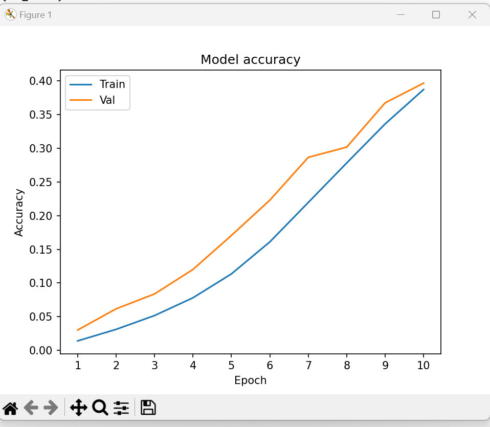
    xx = range(1, len(history.history['accuracy']) + 1)
    plt.plot(xx, history.history['accuracy'])
    plt.plot(xx, history.history['val_accuracy'])
    plt.title('Model accuracy')
    plt.ylabel('Accuracy')
    plt.xlabel('Epoch')
    plt.xticks(xx)
    plt.legend(['Train', 'Val'], loc='upper left')
    plt.show()



if __name__ == '__main__':
    main()

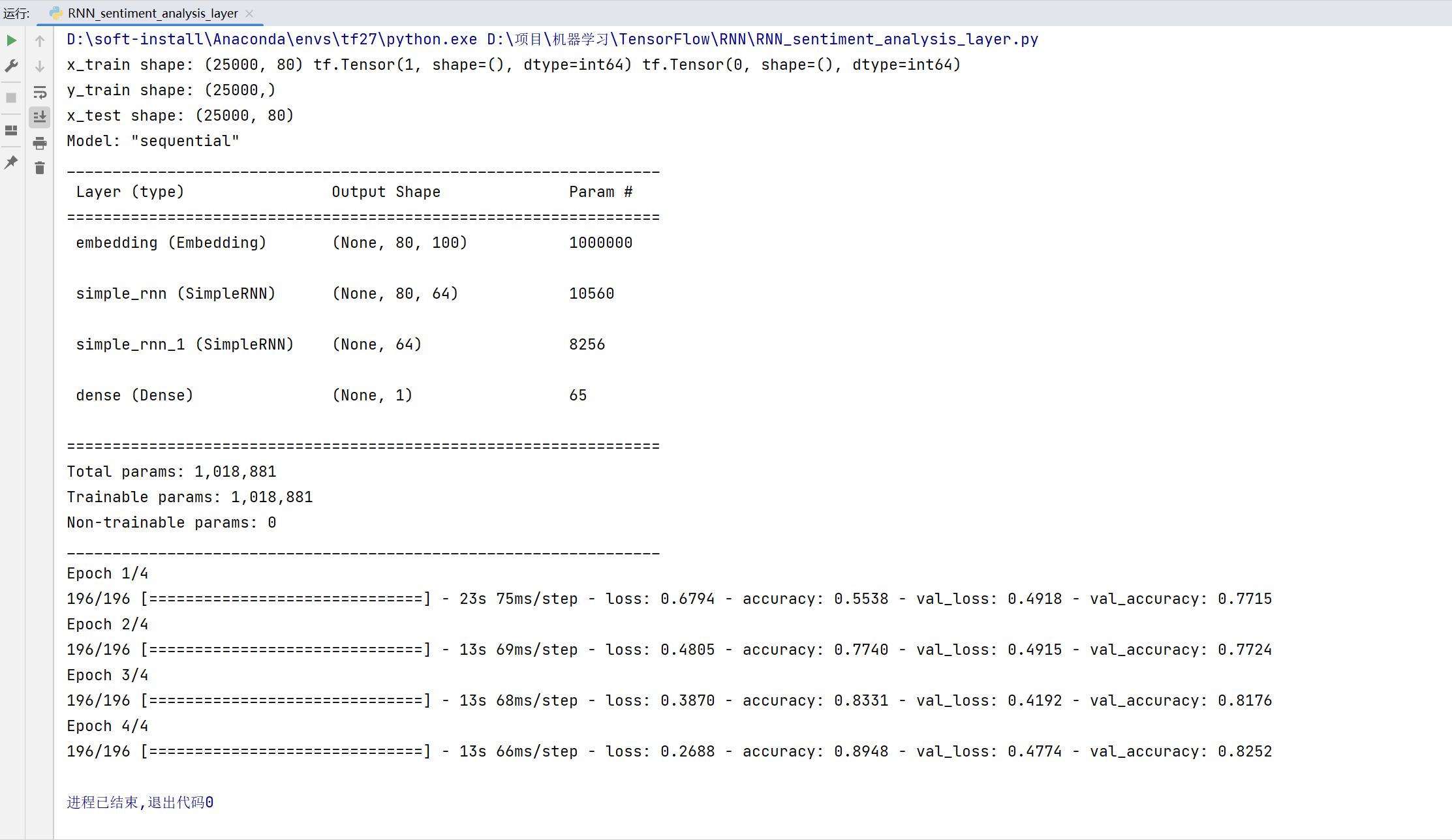
RNN情感分析

import  os
os.environ['TF_CPP_MIN_LOG_LEVEL']='2'

import  tensorflow as tf
import  numpy as np
from    tensorflow import keras
from    tensorflow.keras import layers,Sequential


tf.random.set_seed(22)
np.random.seed(22)
assert tf.__version__.startswith('2.')

batchsz = 128
total_words = 10000
max_review_len = 80
embedding_len = 100
(x_train, y_train), (x_test, y_test) = keras.datasets.imdb.load_data(num_words=total_words)
# x_train:[b, 80]
# x_test: [b, 80]
x_train = keras.preprocessing.sequence.pad_sequences(x_train, maxlen=max_review_len)
x_test = keras.preprocessing.sequence.pad_sequences(x_test, maxlen=max_review_len)


print('x_train shape:', x_train.shape, tf.reduce_max(y_train), tf.reduce_min(y_train))
print('y_train shape:', y_train.shape)
print('x_test shape:', x_test.shape)


model = Sequential([
    layers.Embedding(input_dim=total_words, output_dim=embedding_len, input_length=max_review_len),
    layers.SimpleRNN(64, dropout=0.5, return_sequences=True, unroll=True),
    layers.SimpleRNN(64, dropout=0.5, unroll=True),
    layers.Dense(1,activation='sigmoid')
])


model.build()
model.summary()

model.compile(optimizer = keras.optimizers.Adam(0.001),
        loss=keras.losses.BinaryCrossentropy(), metrics=["accuracy"])

epochs = 4
batch_size = 64
history = model.fit(x_train, y_train, epochs=epochs, batch_size=batchsz,
        validation_data=(x_test, y_test))

LSTM 情感分析

import  os
os.environ['TF_CPP_MIN_LOG_LEVEL']='2'

import  tensorflow as tf
import  numpy as np
from    tensorflow import keras
from    tensorflow.keras import layers,Sequential


tf.random.set_seed(22)
np.random.seed(22)
assert tf.__version__.startswith('2.')

batchsz = 128
total_words = 10000
max_review_len = 80
embedding_len = 100
(x_train, y_train), (x_test, y_test) = keras.datasets.imdb.load_data(num_words=total_words)
# x_train:[b, 80]
# x_test: [b, 80]
x_train = keras.preprocessing.sequence.pad_sequences(x_train, maxlen=max_review_len)
x_test = keras.preprocessing.sequence.pad_sequences(x_test, maxlen=max_review_len)


print('x_train shape:', x_train.shape, tf.reduce_max(y_train), tf.reduce_min(y_train))
print('y_train shape:', y_train.shape)
print('x_test shape:', x_test.shape)


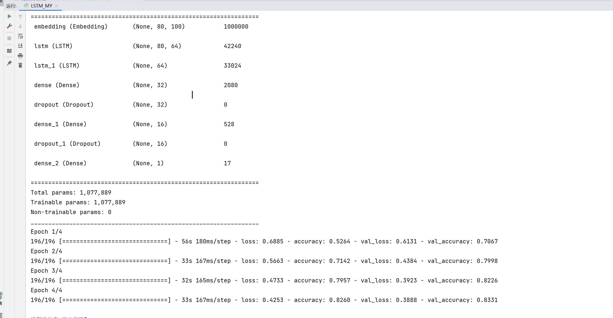
model = Sequential([
    layers.Embedding(input_dim=total_words, output_dim=embedding_len, input_length=max_review_len),
    #layers.LSTM(64, dropout=0.5, return_sequences=True, unroll=True),
    layers.LSTM(64, dropout=0.5, return_sequences=True, unroll=True),
    layers.LSTM(64, dropout=0.5, unroll=True),
    layers.Dense(32, activation=tf.nn.relu),
    layers.Dropout(0.5),
    layers.Dense(16, activation=tf.nn.relu),
    layers.Dropout(0.5),
    layers.Dense(1,activation='sigmoid')
])


model.build()
model.summary()

model.compile(optimizer="Adamax",
        loss=keras.losses.BinaryCrossentropy(), metrics=["accuracy"])

epochs = 4
batch_size = 64
history = model.fit(x_train, y_train, epochs=epochs, batch_size=batchsz,
        validation_data=(x_test, y_test))

其中layers.LSTM的参数可以看这个官方文档
然后这个layers.Embedding:
我们输入的一些词语他都是一维的，这样我们是不能处理的，所以我们要变成二维的，首先想到的一个是one_hot编码。但是这个one_hot编码如果词语多的话会消耗大量的空间。然后就引出了embedding，这个的用处就是降维。
然后他的作用：
就是把稀疏矩阵变成一个密集矩阵，也称为查表，因为他们之间是一个一一映射关系。
这种关系在反向传播的过程中，是一直在更新的，因此能在多次epoch后，使得这个关系变成相对成熟。

例如这个：

model.add(tf.keras.layers.Embedding(1000, 64, input_length=10))
The model will take as input an integer matrix of size (batch,
input_length), and the largest integer (i.e. word index) in the input
should be no larger than 999 (vocabulary size).
Now model.output_shape is (None, 10, 64), where None is the batch
dimension.

import tensorflow as tf
import numpy as np
model = tf.keras.Sequential()
model.add(tf.keras.layers.Embedding(1000, 64, input_length=10))
# The model will take as input an integer matrix of size (batch,
# input_length), and the largest integer (i.e. word index) in the input
# should be no larger than 999 (vocabulary size).
# Now model.output_shape is (None, 10, 64), where `None` is the batch
# dimension.
input_array = np.random.randint(1000, size=(32, 10))
print(input_array)
model.compile('rmsprop', 'mse')
output_array = model.predict(input_array)
print(output_array.shape)

然后执行结果就是变成了[None,10,64]的一个关系矩阵

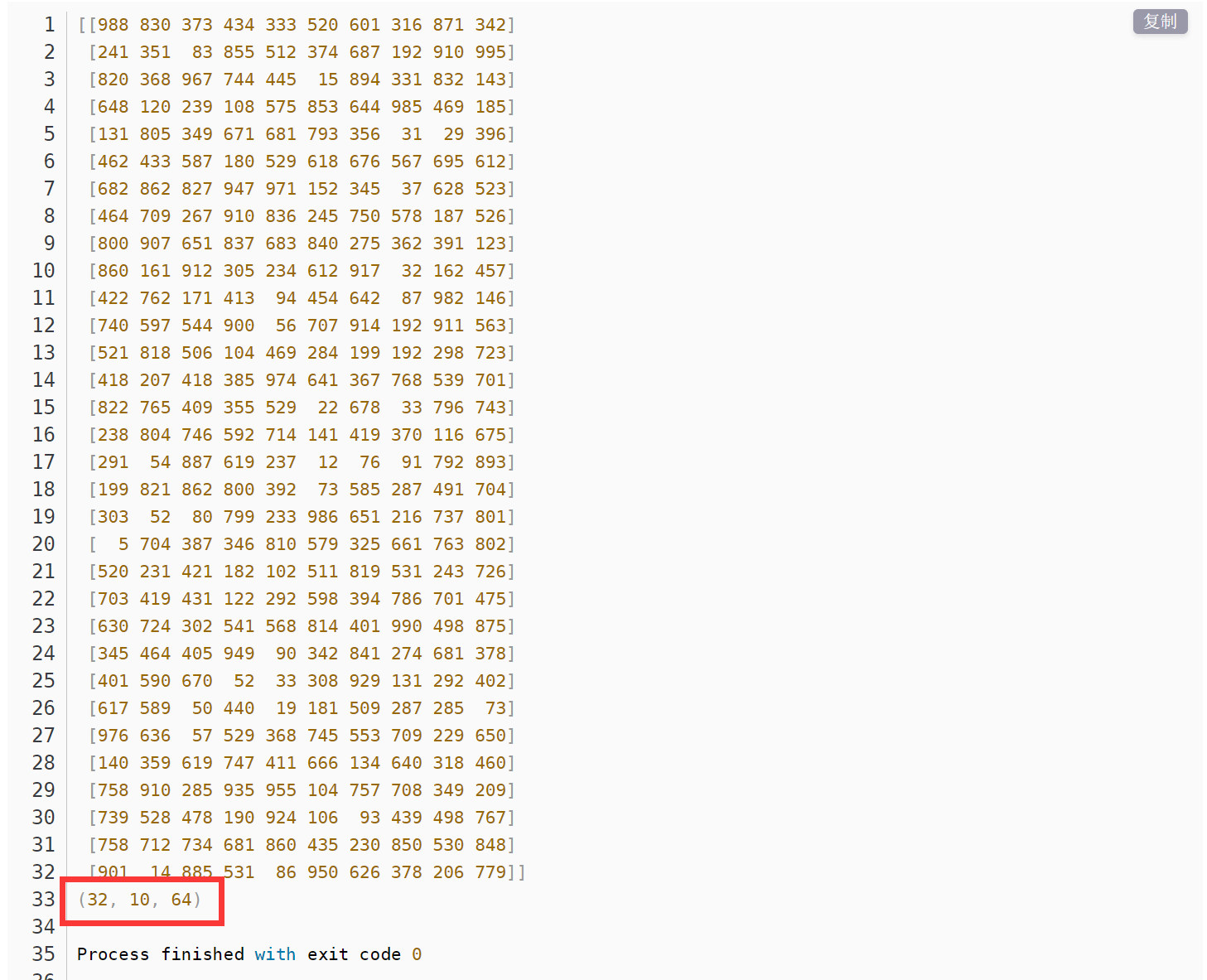
然后看看我们的这个：

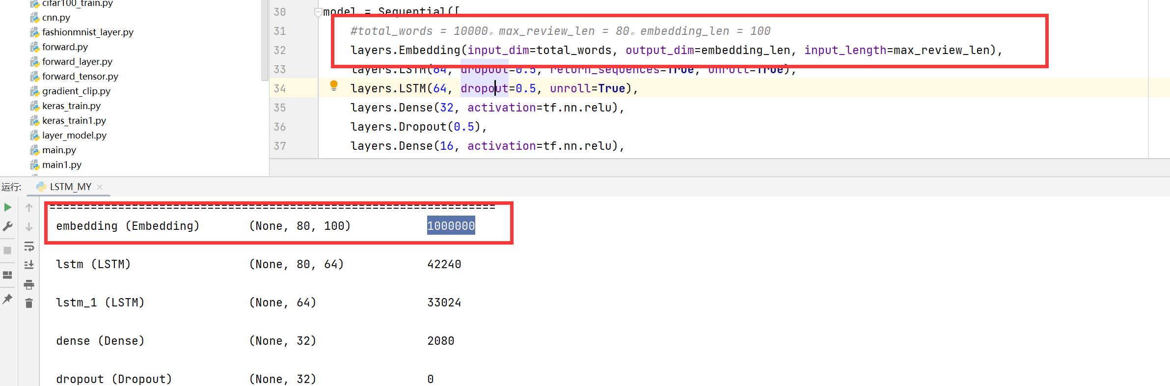
这里第一个input_dim是你的词的大小，output_dim和input_length，就是变成[None,input_length,output_dim]。

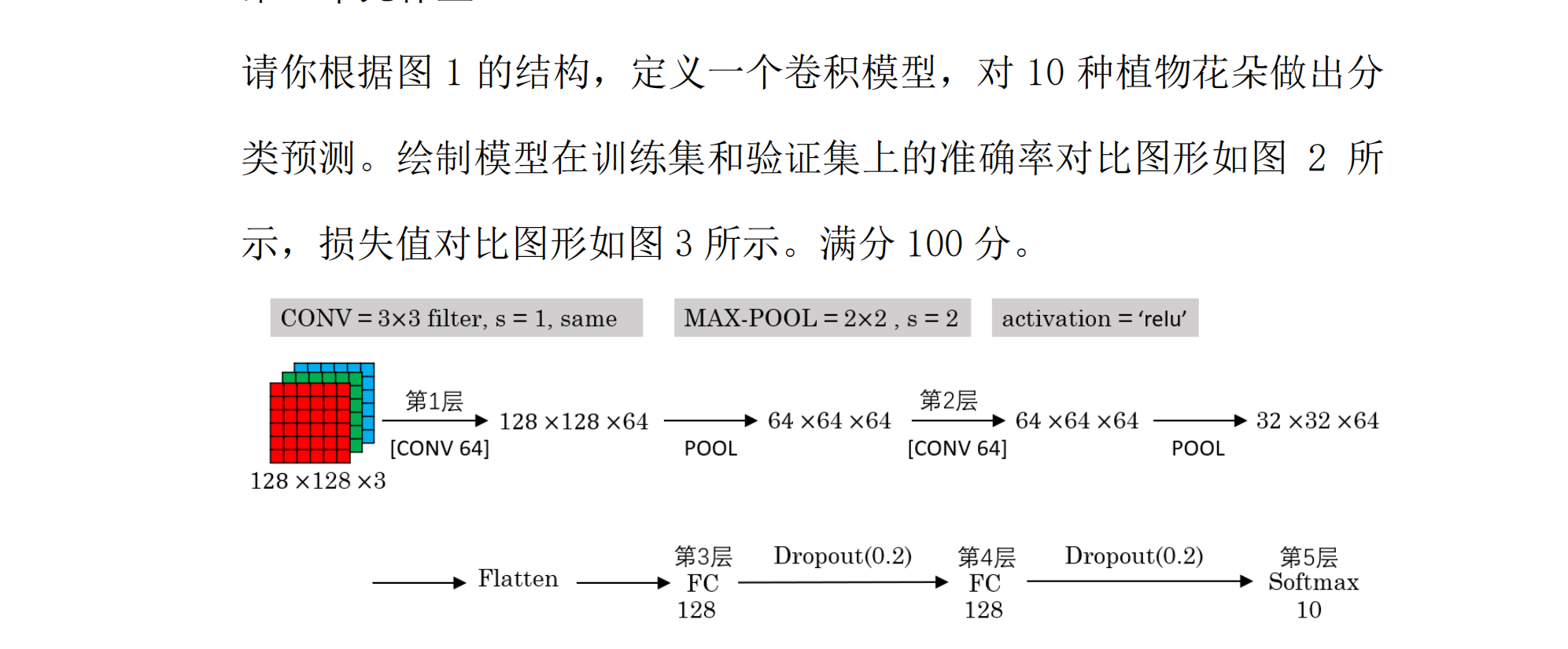
图片花朵识别

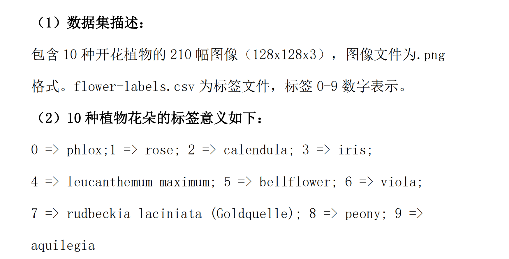
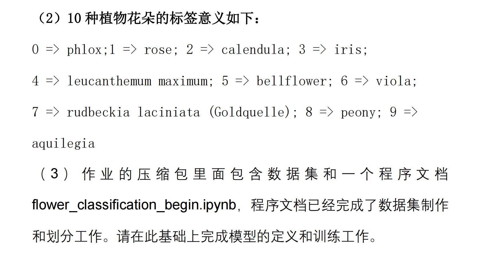
我们看一下这个数据集：

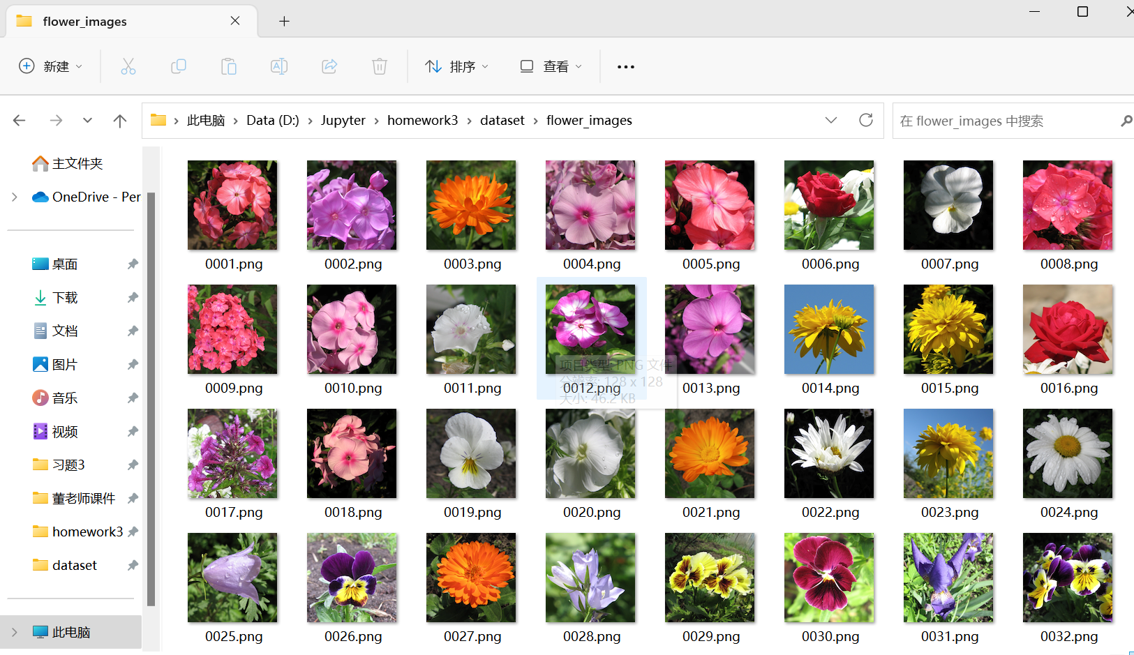
这个主要的是数据集的处理，这个数据集是图片，我们要制作数据集。
这里主要用到了一个API就是：

tf.keras.utils.load_img(
path, grayscale=False, color_mode='rgb', target_size=None,
interpolation='nearest'
)
path 图像文件的路径。
grayscale 不推荐使用 color_mode="grayscale" 。
color_mode "grayscale"、"rgb"、"rgba" 之一。默认值："rgb"。所需的图像格式。
target_size None (默认为原始大小)或整数元组 (img_height, img_width) 。
interpolation 如果目标大小与加载图像的大小不同，则用于重新采样图像的插值方法。支持的方法是"nearest"、"bilinear" 和"bicubic"。如果安装了 PIL 1.1.3 或更高版本，则还支持"lanczos"。如果安装了 PIL 3.4.0 或更高版本，则还支持 "box" 和 "hamming"。默认情况下，使用"nearest"。

然后返回一个 PIL 图像实例。

tf.keras.utils.img_to_array(
img, data_format=None, dtype=None
)
img 输入 PIL Image 实例。

输入 PIL Image 实例。
返回 一个 3D Numpy 数组。

具体用法：

img = keras.utils.load_img("./dataset/flower_images/"+filename,
                               target_size=(128, 128))
x = keras.utils.img_to_array(img)

然后返回的这个就是一个3D的Numpy数组

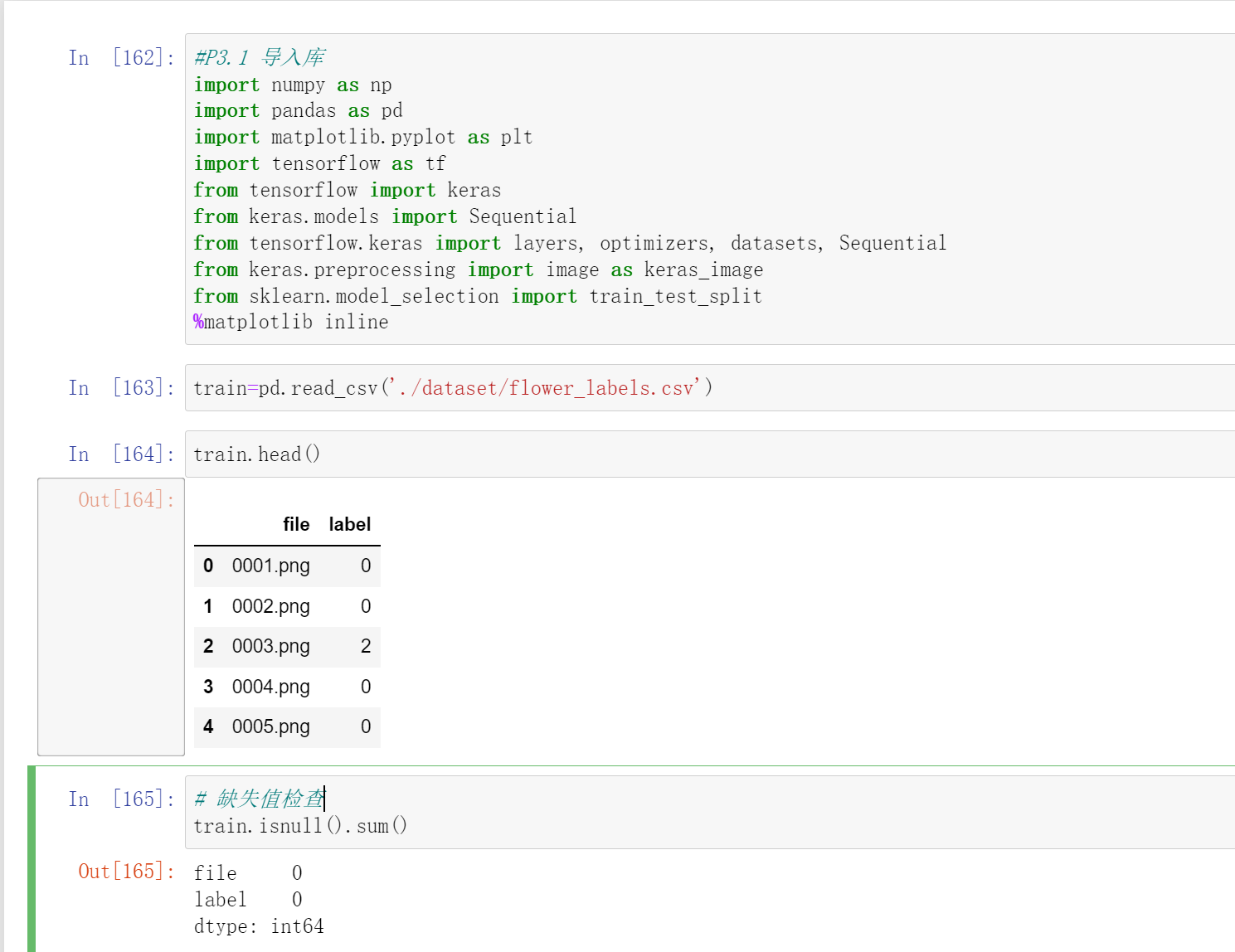
#P3.1 导入库
import numpy as np
import pandas as pd
import matplotlib.pyplot as plt
import tensorflow as tf
from tensorflow import keras
from keras.models import Sequential
from tensorflow.keras import layers, optimizers, datasets, Sequential
from keras.preprocessing import image as keras_image
from sklearn.model_selection import train_test_split
%matplotlib inline
#读取标签列
train=pd.read_csv('./dataset/flower_labels.csv')
train.head()
# 缺失值检查
train.isnull().sum()

%%time
# P3.5 读取图片，制作成numpy
def file_to_tensor(filename):
    img = keras.utils.load_img("./dataset/flower_images/"+filename, 
                               target_size=(128, 128))
    x = keras.utils.img_to_array(img)
    return np.expand_dims(x, axis=0)

def path_to_tensors(img_path):
    list_of_tensors = [file_to_tensor(filename) for filename in img_path]
    return np.vstack(list_of_tensors)

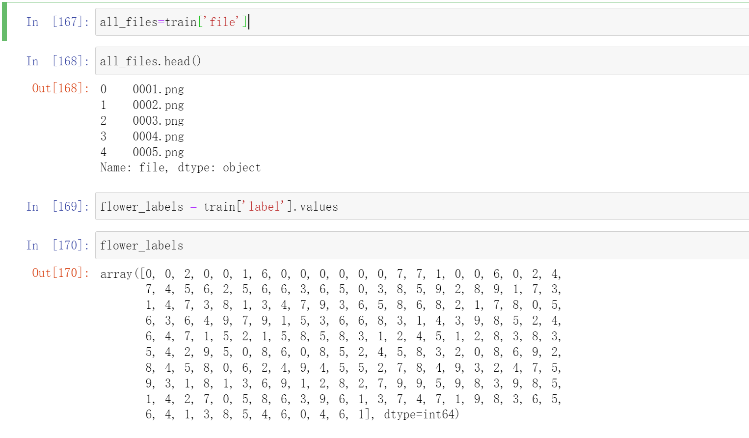
#图片
all_files=train['file']
all_files.head()
#标签
flower_labels = train['label'].values
flower_labels

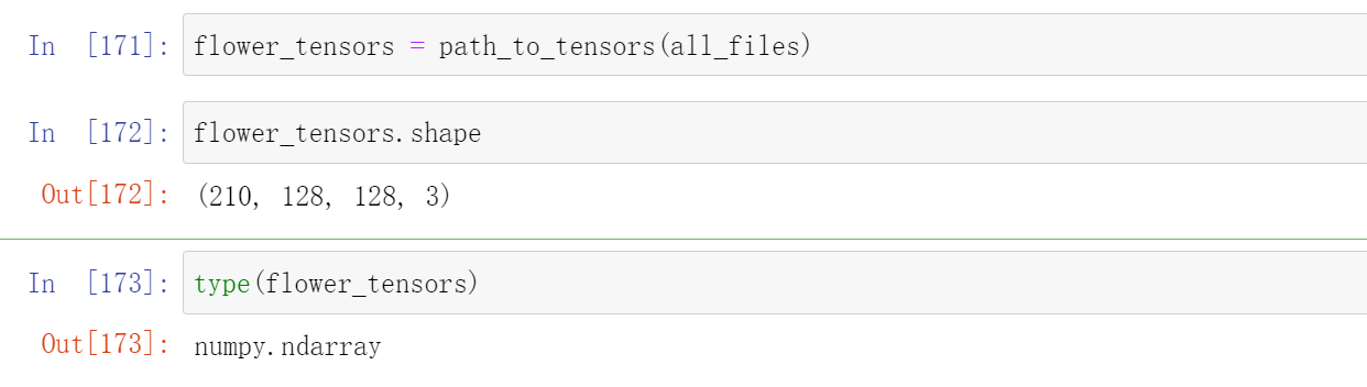
flower_tensors = path_to_tensors(all_files)
flower_tensors.shape
type(flower_tensors)

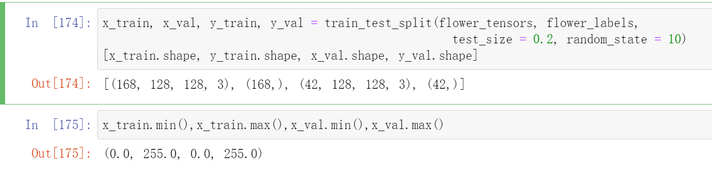
划分数据集、测试集

x_train, x_val, y_train, y_val = train_test_split(flower_tensors, flower_labels,
                                                    test_size = 0.2, random_state = 10)
[x_train.shape, y_train.shape, x_val.shape, y_val.shape]
x_train.min(),x_train.max(),x_val.min(),x_val.max()

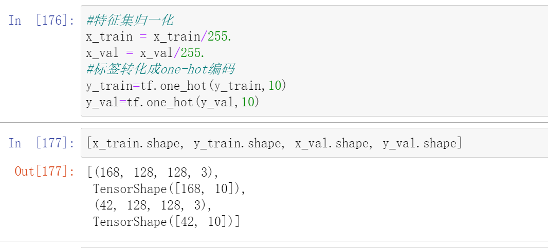
特征集归一化、标签转化成one-hot编码

#特征集归一化
x_train = x_train/255.
x_val = x_val/255.
#标签转化成one-hot编码
y_train=tf.one_hot(y_train,10)
y_val=tf.one_hot(y_val,10)
[x_train.shape, y_train.shape, x_val.shape, y_val.shape]

数据训练

model = Sequential([ # 5 units of conv + max pooling
    # unit 1:64
    layers.Conv2D(64, kernel_size=[3, 3], padding="same", activation=tf.nn.relu),
    layers.MaxPool2D(pool_size=[2, 2], strides=2, padding='same'),

    # unit 2:16
    layers.Conv2D(128, kernel_size=[3, 3], padding="same", activation=tf.nn.relu),
    layers.MaxPool2D(pool_size=[2, 2], strides=2, padding='same'),


    layers.Flatten(),
    layers.Dense(128, activation=tf.nn.relu),
    layers.Dropout(0.2),
    layers.Dense(128, activation=tf.nn.relu),
    layers.Dropout(0.2),
    layers.Dense(10, activation='softmax'),
])

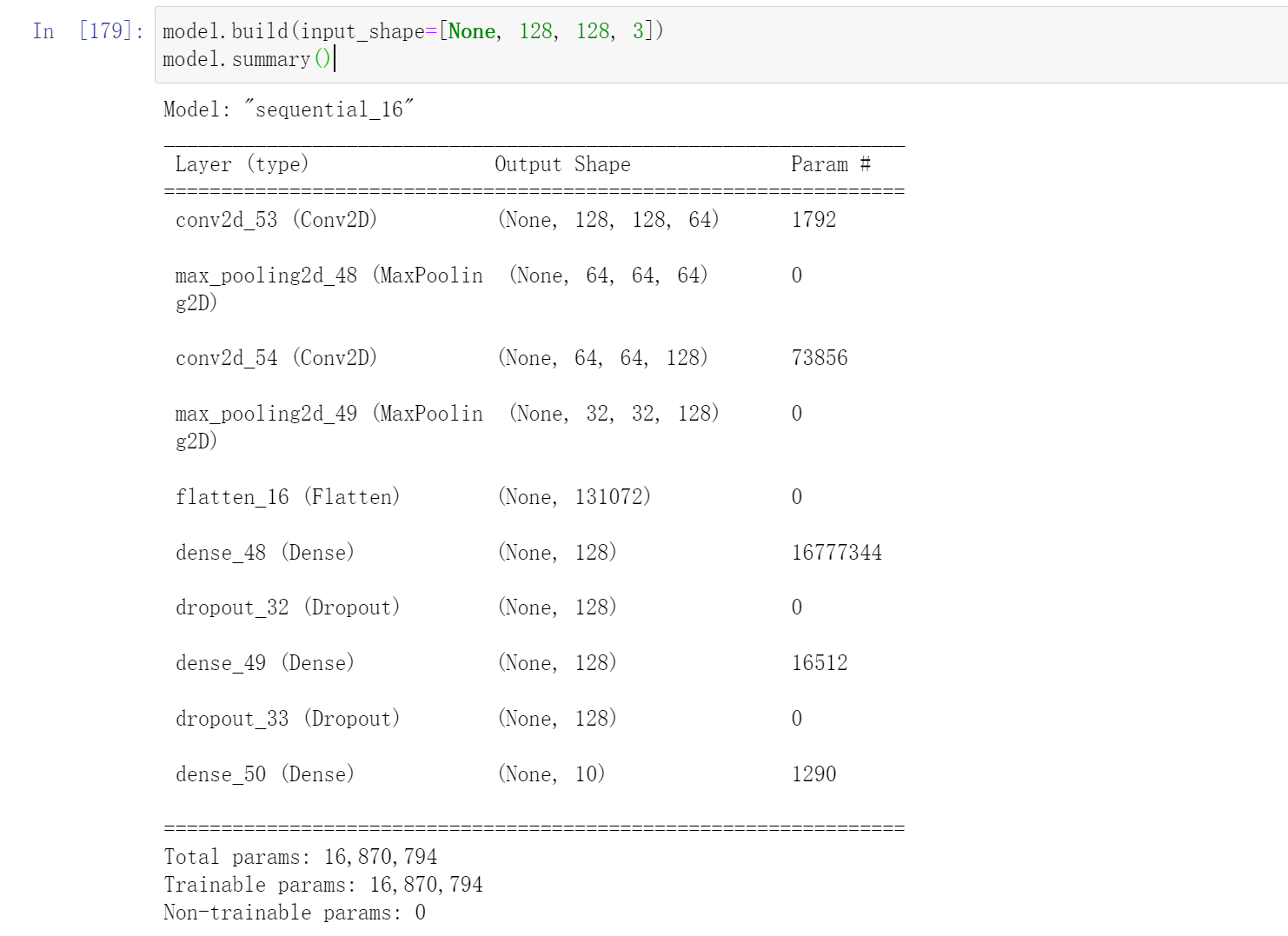
model.build(input_shape=[None, 128, 128, 3])
model.summary()

model.compile(optimizer="Adamax",
                  loss="categorical_crossentropy", metrics=["accuracy"])

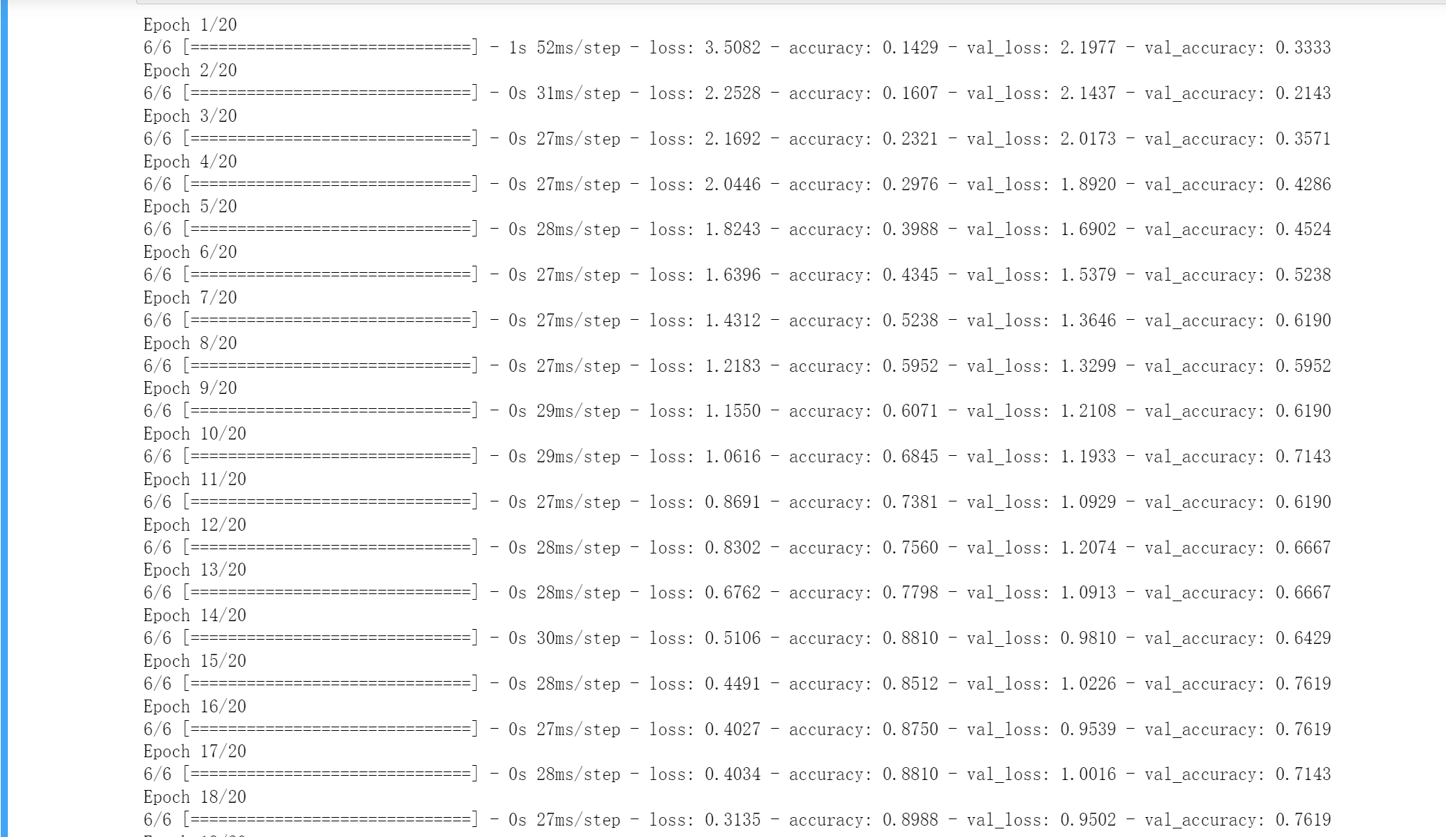
epochs = 20
batch_size = 32
history = model.fit(x_train, y_train, epochs=epochs, batch_size=batch_size,
                validation_data=(x_val, y_val))

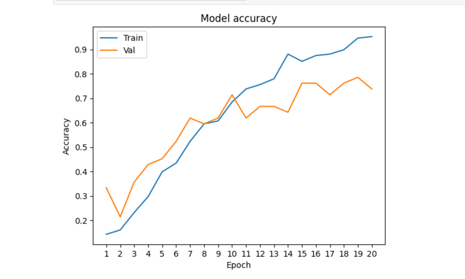
# P3.13绘制准确率与损失值图形--20分，每个10分
x = range(1, len(history.history['accuracy'])+1)
plt.plot(x, history.history['accuracy'])
plt.plot(x, history.history['val_accuracy'])
plt.title('Model accuracy')
plt.ylabel('Accuracy')
plt.xlabel('Epoch')
plt.xticks(x)
plt.legend(['Train', 'Val'], loc='upper left')
plt.show()
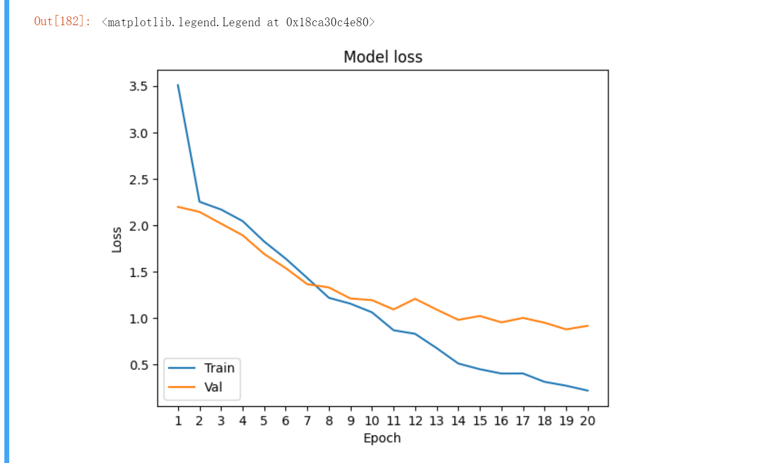
plt.plot(x, history.history['loss'])
plt.plot(x, history.history['val_loss'])
plt.title('Model loss')
plt.ylabel('Loss')
plt.xlabel('Epoch')
plt.xticks(x)
plt.legend(['Train', 'Val'], loc='lower left')

如果你在处理的时候想弄成HDF5数据集的话
用这个

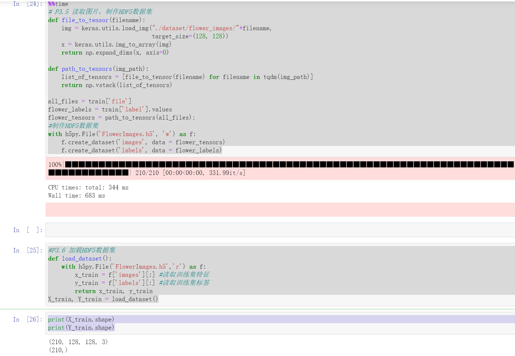
%%time
# P3.5 读取图片，制作HDF5数据集
def file_to_tensor(filename):
    img = keras.utils.load_img("./dataset/flower_images/"+filename, 
                               target_size=(128, 128))
    x = keras.utils.img_to_array(img)
    return np.expand_dims(x, axis=0)

def path_to_tensors(img_path):
    list_of_tensors = [file_to_tensor(filename) for filename in tqdm(img_path)]
    return np.vstack(list_of_tensors)

all_files = train['file']
flower_labels = train['label'].values
flower_tensors = path_to_tensors(all_files);
#制作HDF5数据集
with h5py.File('FlowerImages.h5', 'w') as f:
    f.create_dataset('images', data = flower_tensors)
    f.create_dataset('labels', data = flower_labels)

#P3.6 加载HDF5数据集
def load_dataset():
    with h5py.File('FlowerImages.h5','r') as f:
        x_train = f['images'][:] #读取训练集特征
        y_train = f['labels'][:] #读取训练集标签
        return x_train, y_train
X_train, Y_train = load_dataset()