TensorFlow04-数据集加载

阅读目录

• 1 数据集加载
• 2 tf.keras.datasets（）
  • 2.1 MNIST
  • 2.2 cifar10：CIFAR10小图像分类数据集
• 3 使用tf.data.Dataset.from_tensor_slices五步加载数据集
  • 3.1 tf.data.Dataset.from_tensor_slices()
  • 3.2 使用tf.data.Dataset.from_tensor_slices五步加载数据集
  • 3.3 .shuffe
  • 3.4 .map
  • 3.5 .batch
  • 3.6 .repeat()
• 4 张量测试

 

回到顶部

1 数据集加载

1.karas.datasets(数据加载)
2.tf.data.Dataset.from_tensor_slices(加载成tensor)

• shuffle
• map
• batch
• repeat

回到顶部

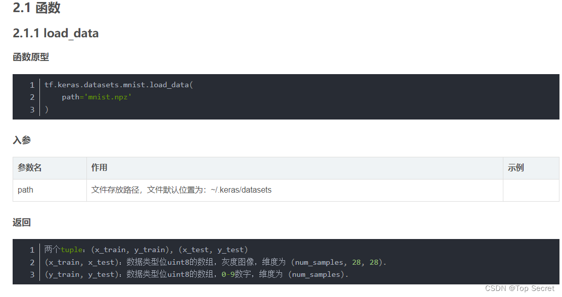
2 tf.keras.datasets（）

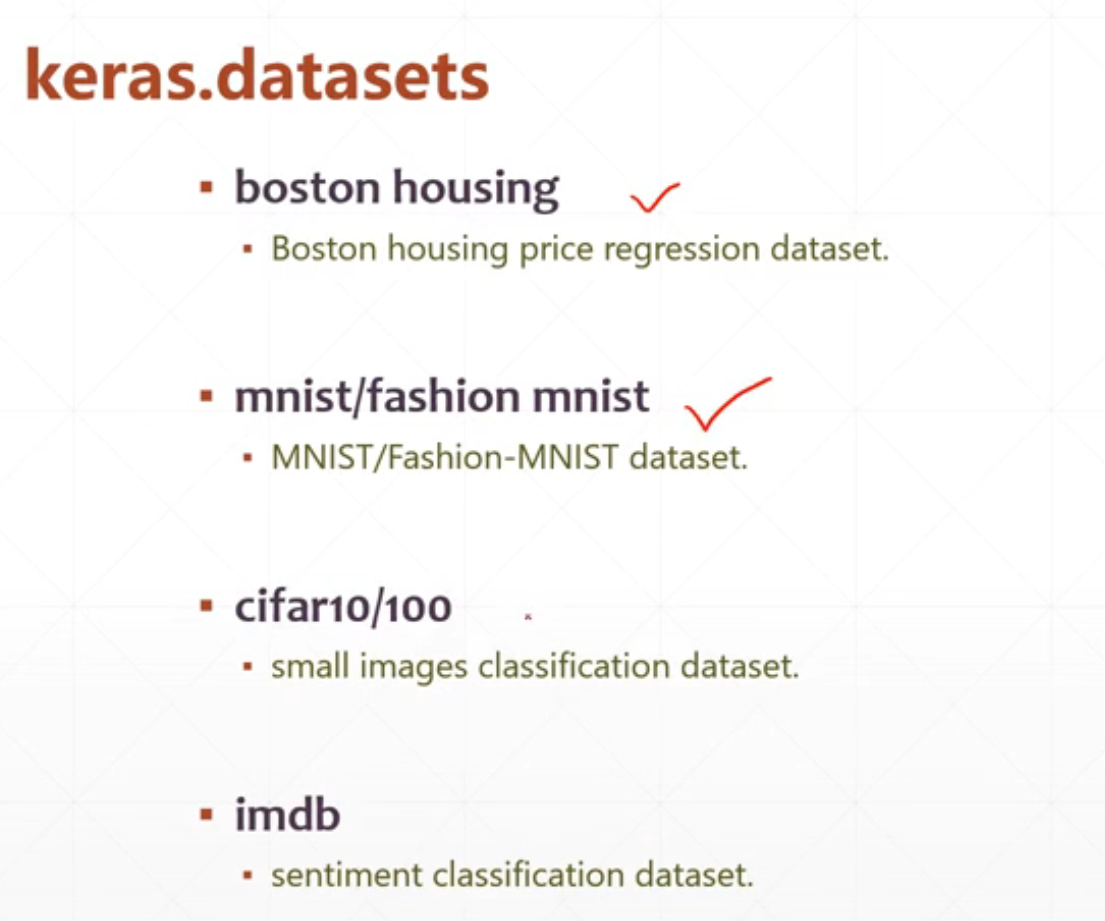
boston_housing：波斯顿房屋价格回归数据集
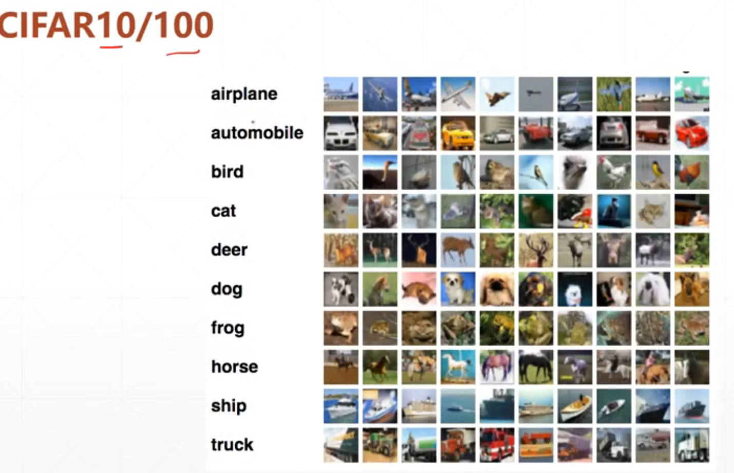
cifar10：CIFAR10小图像分类数据集
cifar100：CIFAR100小图像分类数据集
fashion_mnist：Fashion-MNIST 数据集.
imdb：IMDB 分类数据集,淘宝好评差评
mnist：MNIST手写数字数据集
reuters：路透社主题分类数据集

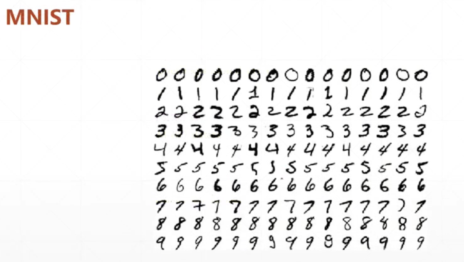
2.1 MNIST

这里主要介绍一下MNIST
是一个28281 ，70k/60k/10k
其中70k是所有的，60k是训练，10k是验证

import tensorflow as tf
from  tensorflow.keras import datasets
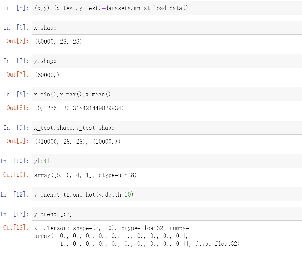
(x,y),(x_test,y_test)=datasets.mnist.load_data()
#这里返回的是一个numpy,（x,y）是训练集，（x_test,y_test）是测试集，x是目标，y是结果

x.shape
#(60000, 28, 28),一共70k

y.shape
#(60000,)

x.min(),x.max(),x.mean()
#(0, 255, 33.318421449829934)
#我们发现这个是0-255,后续我们需要进行标准化，变成[0,1]或者[-1,1],前面我们是用的/255

x_test.shape,y_test.shape
#((10000, 28, 28), (10000,))

y[:4]
#array([5, 0, 4, 1], dtype=uint8)

y_onehot=tf.one_hot(y,depth=10)#这里要把y变成ont_hot码
y_onehot[:2]
#<tf.Tensor: shape=(2, 10), dtype=float32, numpy=
#array([[0., 0., 0., 0., 0., 1., 0., 0., 0., 0.],
#       [1., 0., 0., 0., 0., 0., 0., 0., 0., 0.]], dtype=float32)>

数据集的加载：

2.2 cifar10：CIFAR10小图像分类数据集

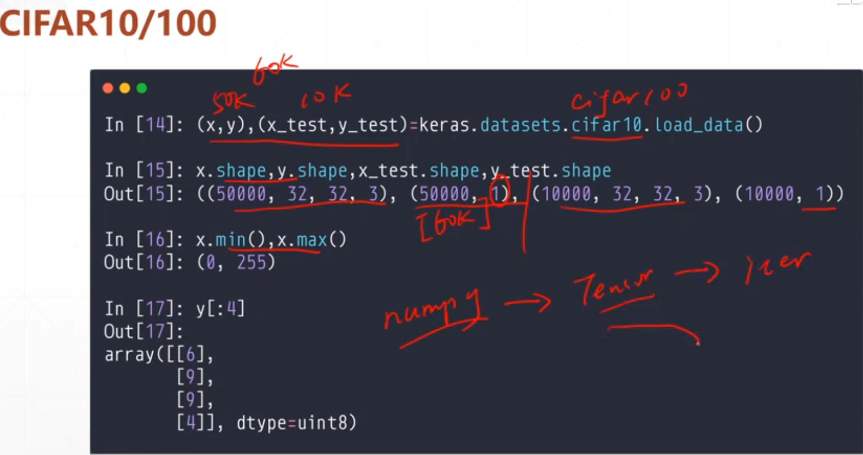
我们拿到这个数据之后基本都是numpy类型的，但是我们需要把他变成numpy->Tensor->iter,这是一个很常见的工作，所以我们那个整合到一个API中了，就是tf.data.Dataset

回到顶部

3 使用tf.data.Dataset.from_tensor_slices五步加载数据集

3.1 tf.data.Dataset.from_tensor_slices()

tf.data.Dataset.from_tensor_slices(
tensors, name=None
)
该函数的作用是接收tensor，对tensor的第一维度进行切分，并返回一个表示该tensor的切片数据集.

获取了这个(x,y),(x_test,y_test)之后我们需要一个迭代器对他进行处理

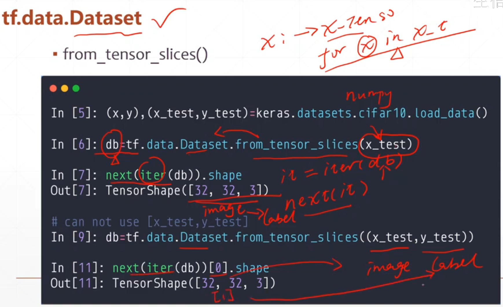
这个比较好的地方就是我们可以对两个数据进行转换，tf.data.Dataset.from_tensor_slices((x_test,y_test))这样next(iter(db))[0]就是第一个x_test,next(iter(db))[1]就是第二个label

3.2 使用tf.data.Dataset.from_tensor_slices五步加载数据集

参考文章：传送门

Step0: 准备要加载的numpy数据
Step1: 使用 tf.data.Dataset.from_tensor_slices() 函数进行加载
Step2: 使用 shuffle() 打乱数据
Step3: 使用 map() 函数进行预处理
Step4: 使用 batch() 函数设置 batch size 值
Step5: 根据需要 使用 repeat() 设置是否循环

import tensorflow as tf
from tensorflow import keras
 
def load_dataset():
	# Step0 准备数据集, 可以是自己动手丰衣足食, 也可以从 tf.keras.datasets 加载需要的数据集(获取到的是numpy数据) 
	# 这里以 mnist 为例
	(x, y), (x_test, y_test) = keras.datasets.mnist.load_data()
	
	# Step1 使用 tf.data.Dataset.from_tensor_slices 进行加载
	db_train = tf.data.Dataset.from_tensor_slices((x, y)）
	db_test = tf.data.Dataset.from_tensor_slices((x_test, y_test))
	
	# Step2 打乱数据
	db_train.shuffle(1000)
	db_test.shuffle(1000)
	
	# Step3 预处理 (预处理函数在下面)
	db_train.map(preprocess)
	db_test.map(preprocess)
 
	# Step4 设置 batch size 一次喂入64个数据
	db_train.batch(64)
	db_test.batch(64)
 
	# Step5 设置迭代次数(迭代2次) test数据集不需要emmm
	db_train.repeat(2)
 
	return db_train, db_test
 
def preprocess(labels, images):
	'''
	最简单的预处理函数:
		转numpy为Tensor、分类问题需要处理label为one_hot编码、处理训练数据
	'''
	# 把numpy数据转为Tensor
	labels = tf.cast(labels, dtype=tf.int32)
	# labels 转为one_hot编码
	labels = tf.one_hot(labels, depth=10)
	# 顺手归一化
	images = tf.cast(images, dtype=tf.float32) / 255
	return labels, images

3.3 .shuffe

这是一个打散函数，就是本来数据集是按照一定顺序的，比如说是0，1，2，3，4，5这样我们需要把这个函数进行打散处理例如变成4，3，5，0，2，1。

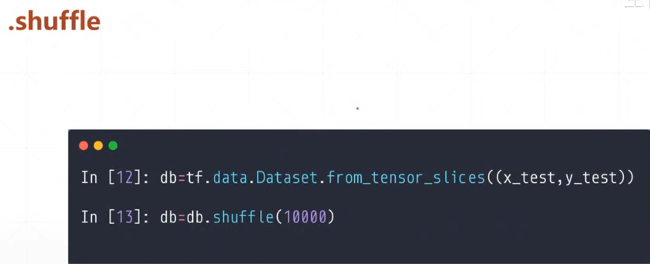
这里面的数shuffle(10000)，我们稍微给大一点就行，没有什么影响的

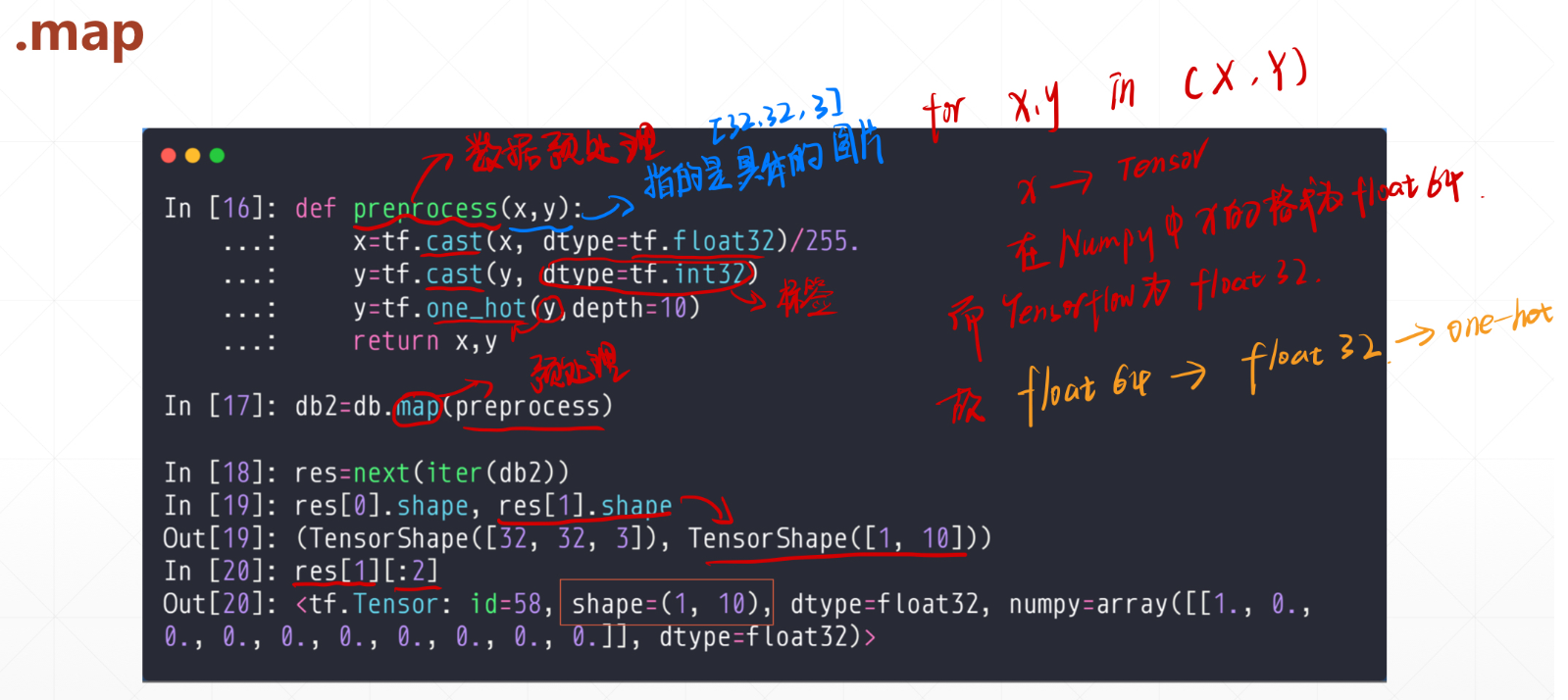
3.4 .map

这里我们需要首先定义一个preprocess函数，然后我们调用db2=db.map(preprocess)这样我们可以对于db中的数据按照preprocess函数进行全部预处理

3.5 .batch

在进行数据操作是我们并不是对数据进行一个一个的处理，而是一个batch一个batch的进行处理，这时候我们需要用的db3=db2.batch(32),这里就是分成32一个batch。

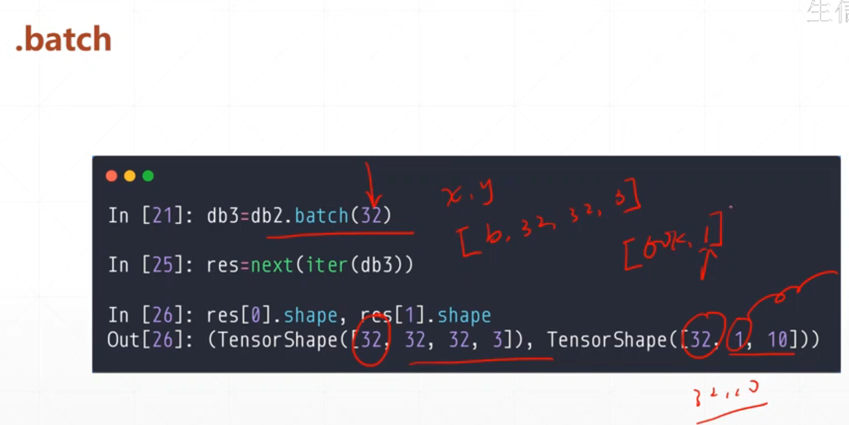
处理完成之后我们就可以调用

for x,y in db3:
      里面返回x[b,32,32,3],y[b,10]
      里面的b是那一捆

如果说我们调用

where True:
    x,y=next(iter())

#这样可能会出现异常

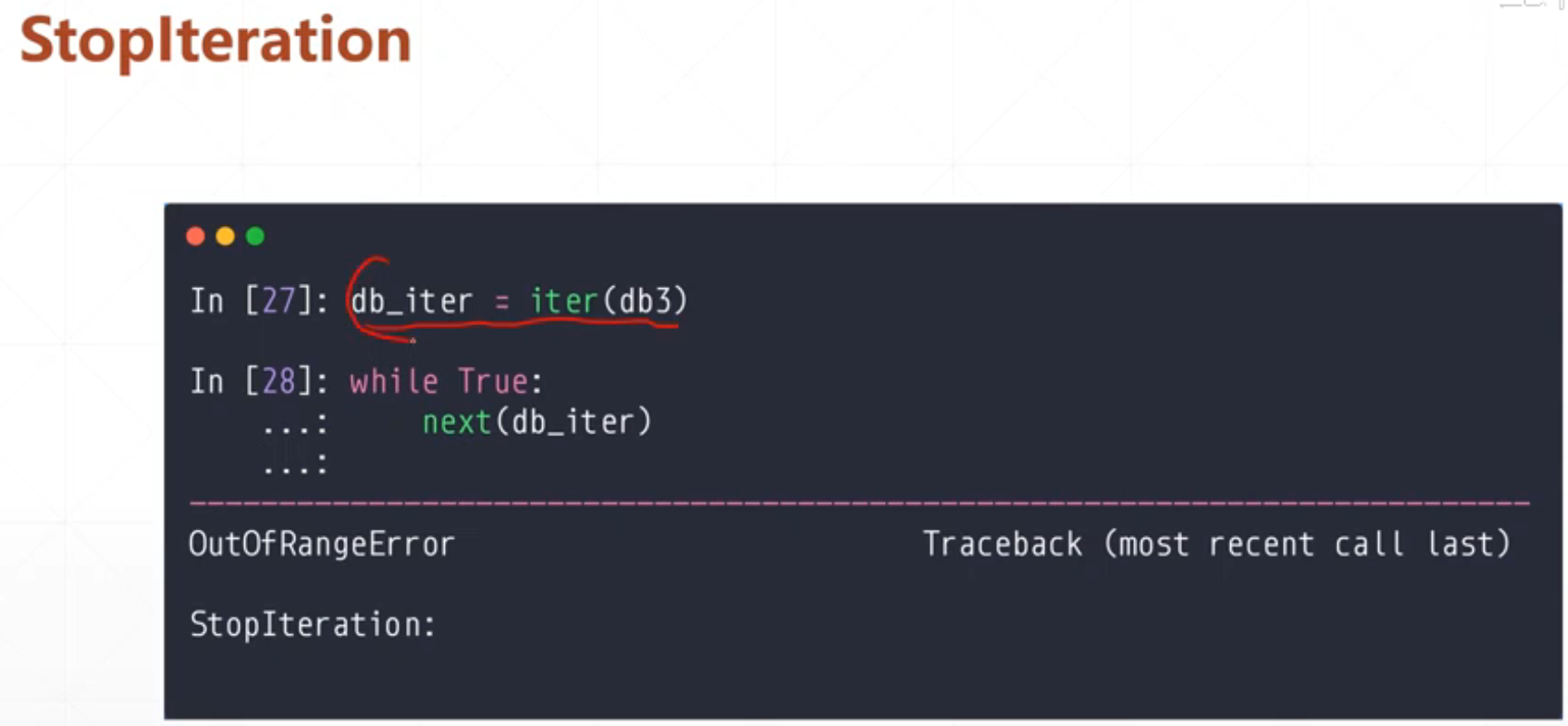
我们在这里如果用到where True的话会有一个异常
我们也可以指定对这个数据集迭代几次

3.6 .repeat()

db4=db3.repeat(k)
这是迭代k次

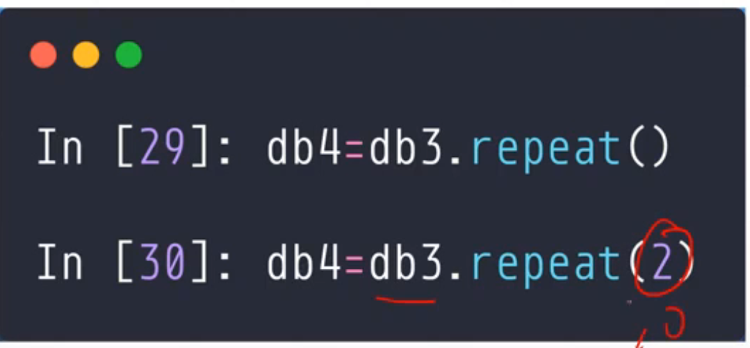
这样我们在调用

for x,y in db4:
	

的时候就不会迭代一次就推出了

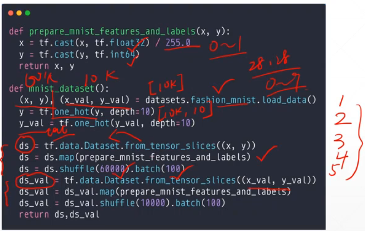
1.这里先加载
2.one_hot
3.转化到Dataset中
4.调用预处理
5.调用shuffle和batch

回到顶部

4 张量测试

这个测试就是我们之前预测了一个模型，然后我们用它测试的模型进行测试正确率

import  tensorflow as tf
from    tensorflow import keras
from    tensorflow.keras import datasets
import  os

os.environ['TF_CPP_MIN_LOG_LEVEL'] = '2'

# x: [60k, 28, 28], [10, 28, 28]
# y: [60k], [10k]
(x, y), (x_test, y_test) = datasets.mnist.load_data()
# x: [0~255] => [0~1.]
x = tf.convert_to_tensor(x, dtype=tf.float32) / 255.
y = tf.convert_to_tensor(y, dtype=tf.int32)
x_test = tf.convert_to_tensor(x_test, dtype=tf.float32) / 255.
y_test = tf.convert_to_tensor(y_test, dtype=tf.int32)

print(x.shape, y.shape, x.dtype, y.dtype)
print(tf.reduce_min(x), tf.reduce_max(x))
print(tf.reduce_min(y), tf.reduce_max(y))


train_db = tf.data.Dataset.from_tensor_slices((x,y)).batch(128)
test_db = tf.data.Dataset.from_tensor_slices((x_test,y_test)).batch(128)
train_iter = iter(train_db)
sample = next(train_iter)
print('batch:', sample[0].shape, sample[1].shape)


# [b, 784] => [b, 256] => [b, 128] => [b, 10]
# [dim_in, dim_out], [dim_out]
w1 = tf.Variable(tf.random.truncated_normal([784, 256], stddev=0.1))
b1 = tf.Variable(tf.zeros([256]))
w2 = tf.Variable(tf.random.truncated_normal([256, 128], stddev=0.1))
b2 = tf.Variable(tf.zeros([128]))
w3 = tf.Variable(tf.random.truncated_normal([128, 10], stddev=0.1))
b3 = tf.Variable(tf.zeros([10]))

lr = 1e-3

for epoch in range(100): # iterate db for 10
    for step, (x, y) in enumerate(train_db): # for every batch
        # x:[128, 28, 28]
        # y: [128]

        # [b, 28, 28] => [b, 28*28]
        x = tf.reshape(x, [-1, 28*28])

        with tf.GradientTape() as tape: # tf.Variable
            # x: [b, 28*28]
            # h1 = x@w1 + b1
            # [b, 784]@[784, 256] + [256] => [b, 256] + [256] => [b, 256] + [b, 256]
            h1 = x@w1 + tf.broadcast_to(b1, [x.shape[0], 256])
            h1 = tf.nn.relu(h1)
            # [b, 256] => [b, 128]
            h2 = h1@w2 + b2
            h2 = tf.nn.relu(h2)
            # [b, 128] => [b, 10]
            out = h2@w3 + b3

            # compute loss
            # out: [b, 10]
            # y: [b] => [b, 10]
            y_onehot = tf.one_hot(y, depth=10)

            # mse = mean(sum(y-out)^2)
            # [b, 10]
            loss = tf.square(y_onehot - out)
            # mean: scalar
            loss = tf.reduce_mean(loss)

        # compute gradients
        grads = tape.gradient(loss, [w1, b1, w2, b2, w3, b3])
        # print(grads)
        # w1 = w1 - lr * w1_grad
        w1.assign_sub(lr * grads[0])
        b1.assign_sub(lr * grads[1])
        w2.assign_sub(lr * grads[2])
        b2.assign_sub(lr * grads[3])
        w3.assign_sub(lr * grads[4])
        b3.assign_sub(lr * grads[5])


        if step % 100 == 0:
            print(epoch, step, 'loss:', float(loss))


    # test/evluation
    # [w1, b1, w2, b2, w3, b3]
    total_correct, total_num = 0, 0
    for step, (x,y) in enumerate(test_db):

        # [b, 28, 28] => [b, 28*28]
        x = tf.reshape(x, [-1, 28*28])

        # [b, 784] => [b, 256] => [b, 128] => [b, 10]
        h1 = tf.nn.relu(x@w1 + b1)
        h2 = tf.nn.relu(h1@w2 + b2)
        out = h2@w3 +b3

        # out: [b, 10] ~ R
        # prob: [b, 10] ~ [0, 1]
        prob = tf.nn.softmax(out, axis=1)
        # [b, 10] => [b]
        # int64!!!
        pred = tf.argmax(prob, axis=1)
        pred = tf.cast(pred, dtype=tf.int32)
        # y: [b]
        # [b], int32
        # print(pred.dtype, y.dtype)
        correct = tf.cast(tf.equal(pred, y), dtype=tf.int32)
        correct = tf.reduce_sum(correct)

        total_correct += int(correct)
        total_num += x.shape[0]

    acc = total_correct / total_num
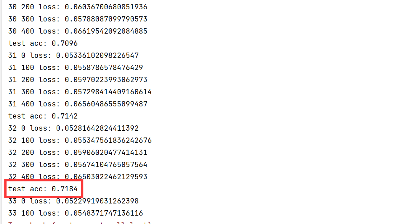
    print('test acc:', acc)

由于我们是三层网络，所以我们最后可能会跑到80%左右