Pandas介绍
1.Pandas介绍
为什么使用Pandas
便捷的数据处理能力
读取文件方便
封装了Matplotlib、Numpy的画图和计算
2.核心数据结构
2.1DataFram
DataFrame
Panel
Series
经常使用的是DataFrame
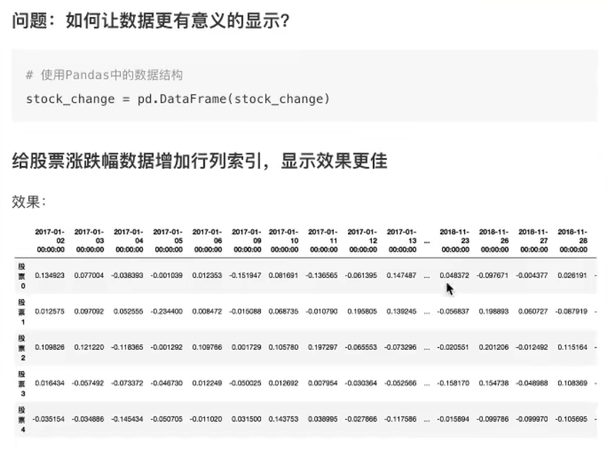
结构:既有行索引,又有列索引的二维数组
使用Pandas中的数据结构
stock_change = pd.DataFrame(stock_change,index= ,columns= )
其中stock_change是numpy类型,index是列索引,cokumns是行索引
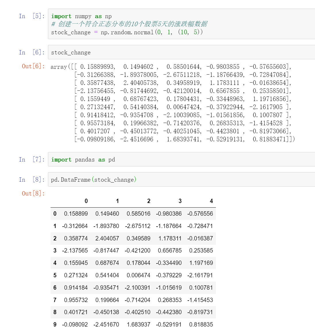
import numpy as np
# 创建一个符合正态分布的10个股票5天的涨跌幅数据
stock_change = np.random.normal(0, 1, (10, 5))
stock_change
array([[-0.07726903,  0.40607587,  1.26740233,  1.48676212, -1.35987104],
       [ 0.28361364,  0.43101642, -0.77154311,  0.48286211, -0.30724683],
       [-0.98583786, -1.96339732,  0.31658224, -1.96541561, -0.39274454],
       [ 2.38020637,  1.47056011, -0.45253103, -0.77381961,  0.4822656 ],
       [ 2.05044671, -0.0743407 ,  0.10900497,  0.00982431, -0.06639766],
       [-1.62883603,  2.370443  , -0.14230101, -1.73515932,  1.6128039 ],
       [ 0.59420384,  0.09903473, -2.82975368,  0.63599429, -0.40809638],
       [ 1.27884397, -0.42832722,  1.07118356, -0.04453698, -0.19217219],
       [ 0.35350472, -0.73933626,  0.81653138, -0.40873922,  1.24391025],
       [-0.66201232, -0.53088568, -2.01276069,  0.03709581,  0.86862061]])
import pandas as pd
pd.DataFrame(stock_change)
	    0	         1	        2	        3           4
0	-0.077269	0.406076	1.267402	1.486762	-1.359871
1	0.283614	0.431016	-0.771543	0.482862	-0.307247
2	-0.985838	-1.963397	0.316582	-1.965416	-0.392745
3	2.380206	1.470560	-0.452531	-0.773820	0.482266
4	2.050447	-0.074341	0.109005	0.009824	-0.066398
5	-1.628836	2.370443	-0.142301	-1.735159	1.612804
6	0.594204	0.099035	-2.829754	0.635994	-0.408096
7	1.278844	-0.428327	1.071184	-0.044537	-0.192172
8	0.353505	-0.739336	0.816531	-0.408739	1.243910
9	-0.662012	-0.530886	-2.012761	0.037096	0.868621
2.1.1DataFrame添加行列索引
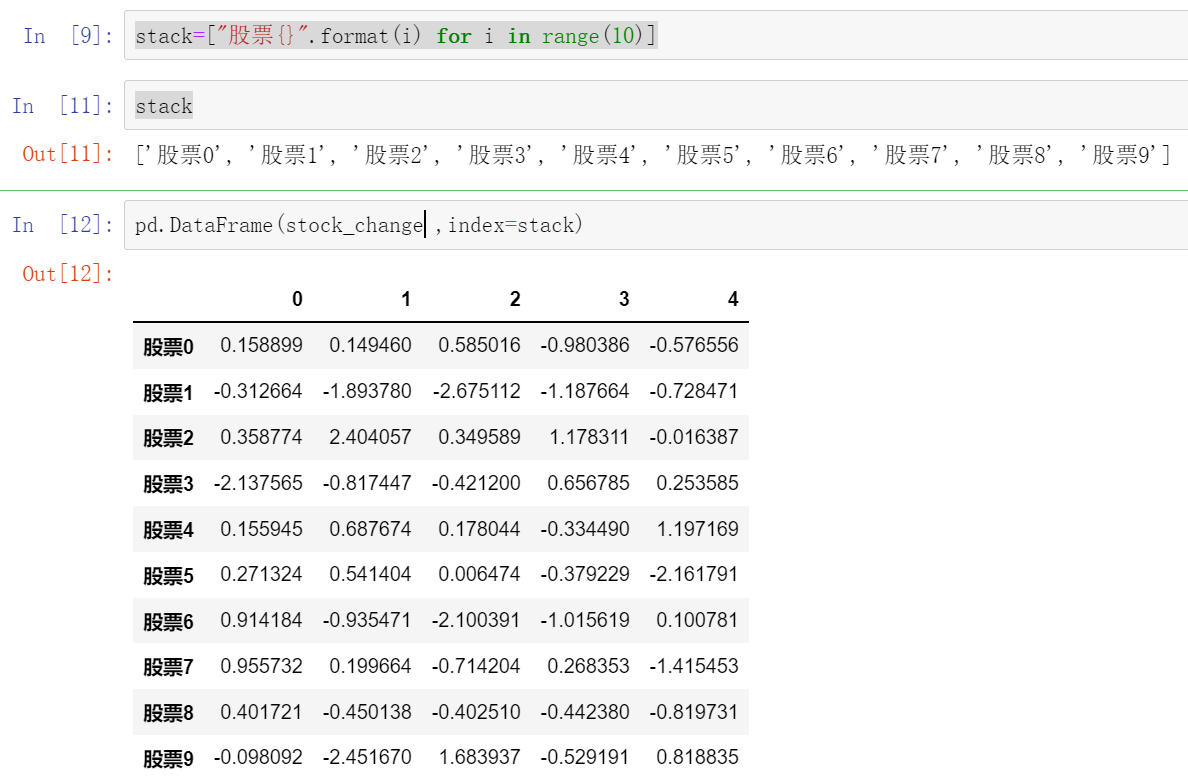
(1)添加行索引
stock是一个列表
pd.DataFrame(stock_change,index=stock)
stack=["股票{}".format(i) for i in range(10)]
stack
['股票0', '股票1', '股票2', '股票3', '股票4', '股票5', '股票6', '股票7', '股票8', '股票9']
pd.DataFrame(stock_change ,index=stack)
	      0	          1	         2	           3	            4
股票0	0.158899	0.149460	0.585016	-0.980386	-0.576556
股票1	-0.312664	-1.893780	-2.675112	-1.187664	-0.728471
股票2	0.358774	2.404057	0.349589	1.178311	-0.016387
股票3	-2.137565	-0.817447	-0.421200	0.656785	0.253585
股票4	0.155945	0.687674	0.178044	-0.334490	1.197169
股票5	0.271324	0.541404	0.006474	-0.379229	-2.161791
股票6	0.914184	-0.935471	-2.100391	-1.015619	0.100781
股票7	0.955732	0.199664	-0.714204	0.268353	-1.415453
股票8	0.401721	-0.450138	-0.402510	-0.442380	-0.819731
股票9	-0.098092	-2.451670	1.683937	-0.529191	0.818835
添加列索引
pd.DataFram(stock_change,index=stack,columns=data)
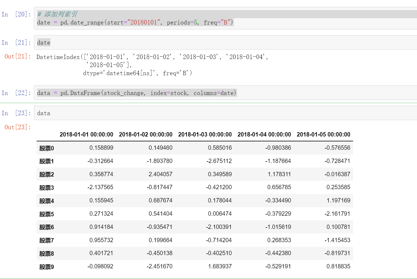
#添加列索引,这个是pandas中的时间序列
date = pd.date_range(start="20180101", periods=5, freq="B")
date
DatetimeIndex(['2018-01-01', '2018-01-02', '2018-01-03', '2018-01-04',
               '2018-01-05'],
              dtype='datetime64[ns]', freq='B')
data = pd.DataFrame(stock_change, index=stock, columns=date)
data
	2018-01-01 00:00:00	2018-01-02 00:00:00	2018-01-03 00:00:00	2018-01-04 00:00:00	2018-01-05 00:00:00
股票0	0.158899	0.149460	0.585016	-0.980386	-0.576556
股票1	-0.312664	-1.893780	-2.675112	-1.187664	-0.728471
股票2	0.358774	2.404057	0.349589	1.178311	-0.016387
股票3	-2.137565	-0.817447	-0.421200	0.656785	0.253585
股票4	0.155945	0.687674	0.178044	-0.334490	1.197169
股票5	0.271324	0.541404	0.006474	-0.379229	-2.161791
股票6	0.914184	-0.935471	-2.100391	-1.015619	0.100781
股票7	0.955732	0.199664	-0.714204	0.268353	-1.415453
股票8	0.401721	-0.450138	-0.402510	-0.442380	-0.819731
股票9	-0.098092	-2.451670	1.683937	-0.529191	0.818835
2.1.2DataFram属性和方法
(1)shape
data.shape
#结果
(10,5)
(2)index(获取列索引)
data.index
Index(['股票0', '股票1', '股票2', '股票3', '股票4', '股票5', '股票6', '股票7', '股票8', '股票9'], dtype='object')
(3)columns(获取行索引)
data.columns
DatetimeIndex(['2018-01-01', '2018-01-02', '2018-01-03', '2018-01-04',
               '2018-01-05'],
              dtype='datetime64[ns]', freq='B')
(4)vlaue(获取里面的array)
data.values
array([[ 0.15889893,  0.1494602 ,  0.58501644, -0.9803855 , -0.57655603],
       [-0.31266388, -1.89378005, -2.67511218, -1.18766439, -0.72847084],
       [ 0.35877438,  2.40405738,  0.34958919,  1.1783111 , -0.01638654],
       [-2.13756455, -0.81744692, -0.42120014,  0.6567855 ,  0.25358501],
       [ 0.1559449 ,  0.68767423,  0.17804431, -0.33448963,  1.19716856],
       [ 0.27132447,  0.54140384,  0.00647424, -0.37922944, -2.1617905 ],
       [ 0.91418412, -0.9354708 , -2.10039085, -1.01561856,  0.1007807 ],
       [ 0.95573184,  0.19966382, -0.71420376,  0.26835313, -1.4154528 ],
       [ 0.4017207 , -0.45013772, -0.40251045, -0.4423801 , -0.81973066],
       [-0.09809186, -2.4516696 ,  1.68393741, -0.52919131,  0.81883471]])
(5).T(转置)
方法
(1)data.head()
默认返回前5行,可以指定data.head(3),前三行
(2)data.tail()
默认返回后5行,可以指定data.tail(3)返回后三行、
2.1.3DataFrame索引的设置
(1)修改行、列索引值
注意:以下修改方式是错误的
错误修改方式
data.index[3] ='股票_3'
正确的方式:
stock_ = ["股票_{}".format(i) for i in range(10)]
data.index=stock_
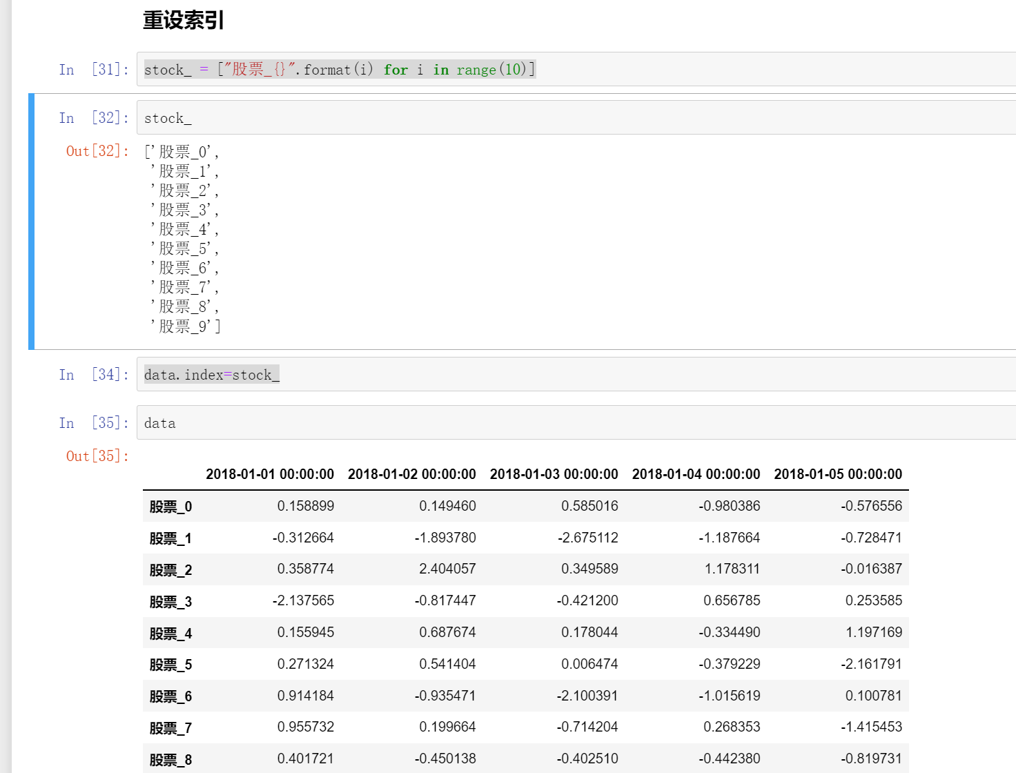
注意不能单独设置索引只能全部修改
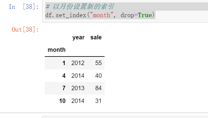
(2)设置新索引
以某列值设置为新的索引
set_index(keys,drop=True)
----keys:列索引名成或者列索引名称的列表
----drop:boolgan,default True.当做新的索引,删除原来的列
df = pd.DataFrame({'month': [1, 4, 7, 10],
'year': [2012, 2014, 2013, 2014],
'sale':[55, 40, 84, 31]})
# 以月份设置新的索引
df.set_index("month", drop=True)
# 设置多个索引,以年和月份
new_df = df.set_index(["year", "month"])
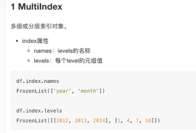
索引的名字:
new_df.index.names
FrozenList(['year', 'month'])
索引数据
new_df.index.levels
FrozenList([[2012, 2013, 2014], [1, 4, 7, 10]])
2.1.4MultiIndex
2.2Panel
pandas.Panel(data=None, items=None, major_axis=None, minor_axis=None,copy=False, dtype=None)存储3维数组的Panel结构

这个是不能查看其结构的,因为其是三维的,但是可以看具体的一维的数据
p = pd.Panel(np.arange(24).reshape(4,3,2),
                 items=list('ABCD'),
                 major_axis=pd.date_range('20130101', periods=3),
                 minor_axis=['first', 'second'])

<class 'pandas.core.panel.Panel'>
Dimensions: 4 (items) x 3 (major_axis) x 2 (minor_axis)
Items axis: A to D
Major_axis axis: 2013-01-01 00:00:00 to 2013-01-03 00:00:00
Minor_axis axis: first to second

p['A']
	      first	  second
2013-01-01	 0	   1
2013-01-02	 2	   3
2013-01-03	 4	   5

p.major_xs("2013-01-01")
	A	B	C	D
first	0	6	12	18
second	1	7	13	19

p.minor_xs("first")

A	B	C	D
2013-01-01	0	6	12	18
2013-01-02	2	8	14	20
2013-01-03	4	10	16	22
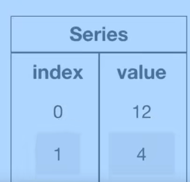
2.3Series
带索引的一维数组
2.3.1创建Series
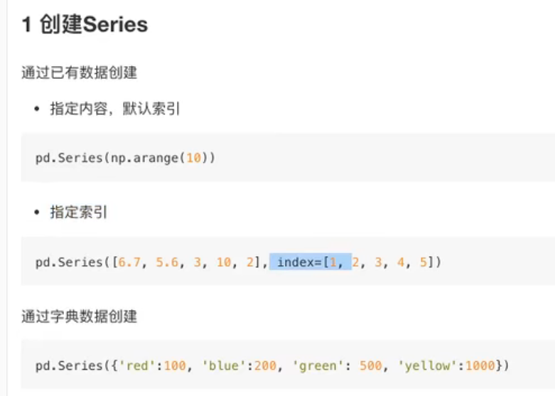
pd.Series([],index=[])
也可以使用字典创建pd.Series({ , , , })
pd.Series([6.7,5.6,3,10,2],index=['a','b','c','d','e'])
a     6.7
b     5.6
c     3.0
d    10.0
e     2.0
dtype: float64
pd.Series(np.arange(3,9,2))
0    3
1    5
2    7
dtype: int32

pd.Series({'red':100, 'blue':200, 'green': 500, 'yellow':1000})
red        100
blue       200
green      500
yellow    1000
dtype: int64
2.3.1Series的属性和方法
属性:
index
value
2.4基本数据操作
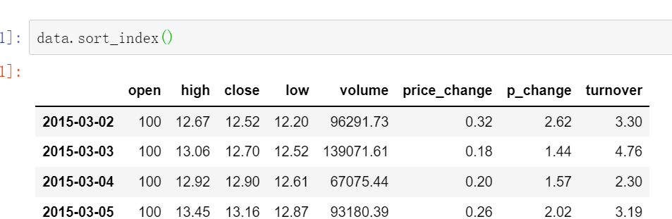
pandas读取数据
data = pd.read_csv("./stock_day/stock_day.csv")
data
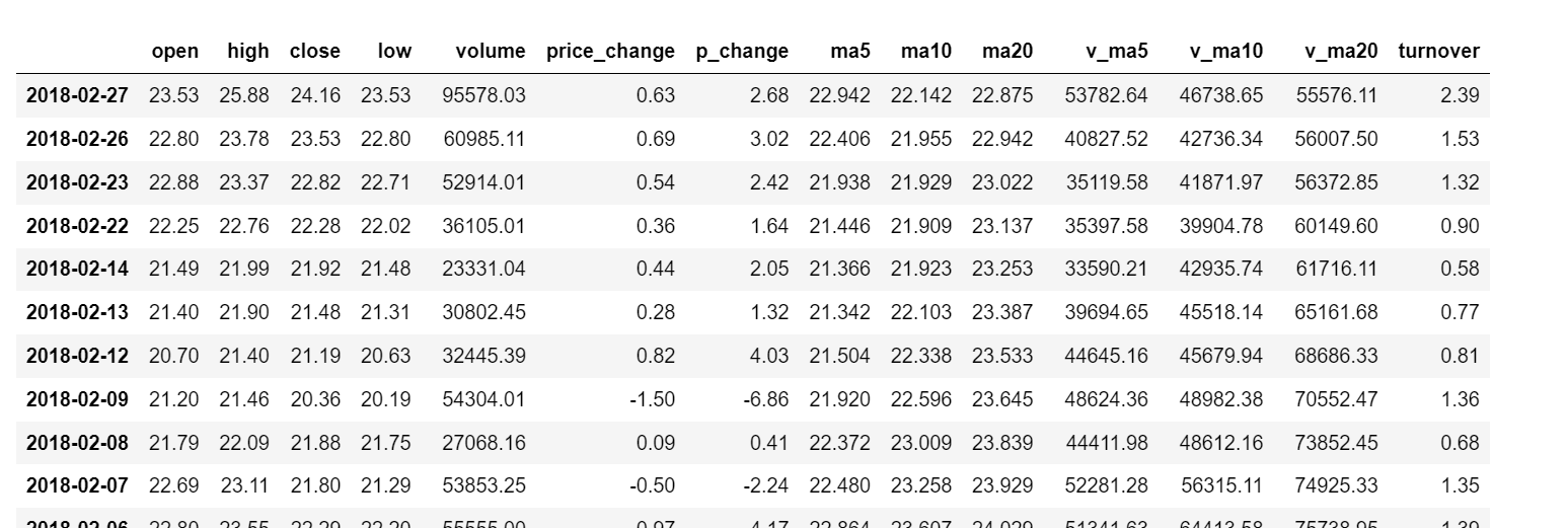
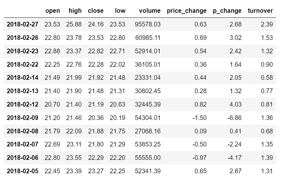
去除一些行
data = data.drop(["ma5","ma10","ma20","v_ma5","v_ma10","v_ma20"], axis=1)
2.4.1索引操作
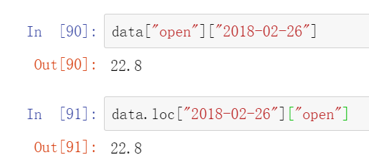
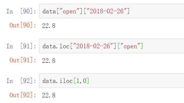
(1)直接索引
这个必须先列后行
对于numpy可以直接索引stock_name[1,1]
但是DataFram不行需要加上索引值data["open"]["2018-02-26"]
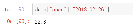
注意这个必须先列后行
(2)按名字索引
data.loc[][]和
这个可以先行后列
data.loc["2018-02-26"]["open"]
(3)按数字索引
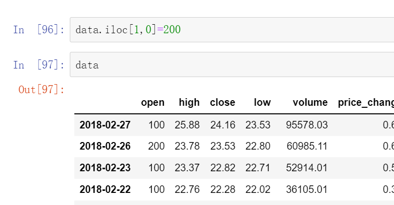
data.iloc[1,0]
这是第一行第0列的那个数字
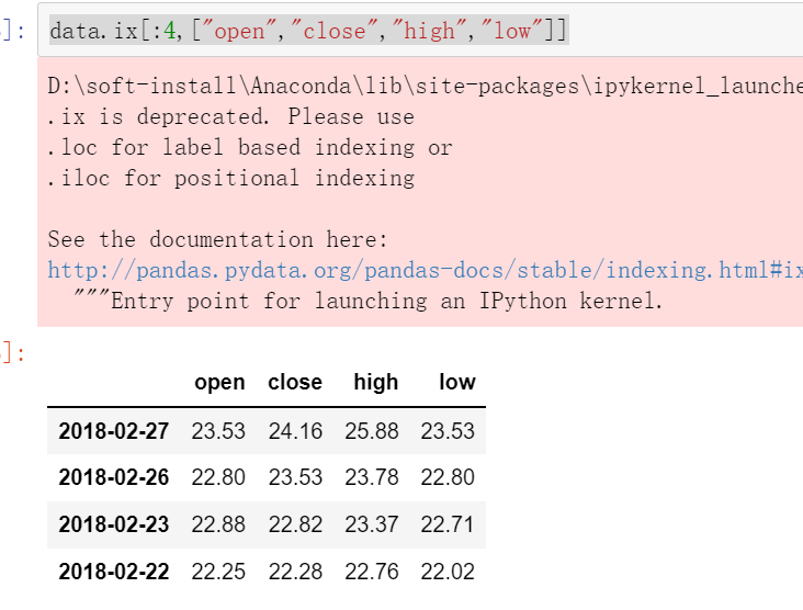
(4)ix组合索引
使用.ix组合索引,这个数字、字母都可以用到
获取行第1天到第4天,['open', 'close', 'high' , 'low']这个四个指标的结果
data.ix[:4,["open","close","high","low"]]
这个ix已经过时了,所以推荐使用loc和iloc
data.loc[data.index[0:4],['open','close','high','low']]
data.iloc[0:4,data.columns.get_indexer(['open','close','high','low'])
2.4.2 赋值操作
(1)对一行全部赋值:
data.open=100
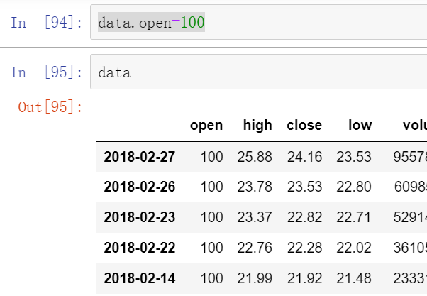
对某一个进行赋值
用前面的索引的方式找到之后进行赋值就行
data.iloc[1,0]=222
2.4.3排序
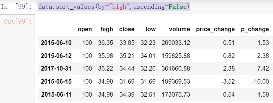
一.DataFrame
(1)对内容进行排序
DataFrame
使用df.sort_values(key=, ascending=)
---key是哪一行、列的索引名称,可以是一个列表,如果第一个相等就按照第二个进行排序
---单个键或者多个键进行排序,默认升序
---ascending=False:降序
---ascending=True:升序
data.sort_values(by="high")
data.sort_values(by="high",ascending=False)
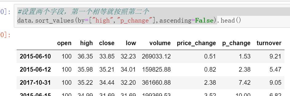
#设置两个字段,第一个相等就按照第二个
data.sort_values(by=["high","p_change"],ascending=False)
(2)对索引进行排序
使用df.sort_index()对索引进行排序
这个股票的日期索引原来是从大到小,现在重新排序,从小到大
二.Series
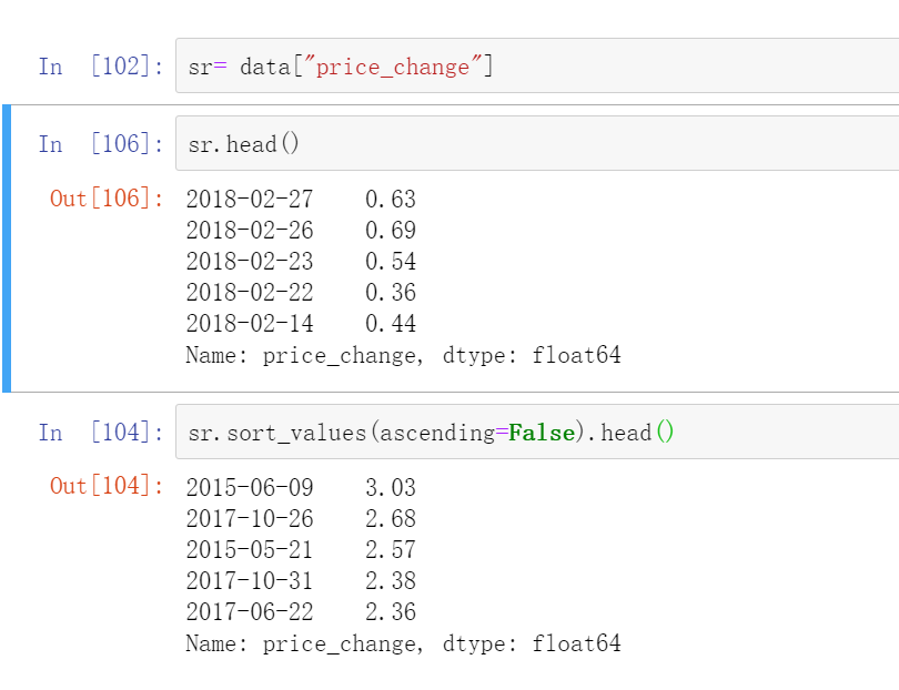
(1)内容进行排序
使用Series.sort_values(ascending=True)对内容进行排序
Series排序时,只有一列,不需要参数
sr= data["price_change"]
sr.head()
2018-02-27    0.63
2018-02-26    0.69
2018-02-23    0.54
2018-02-22    0.36
2018-02-14    0.44
Name: price_change, dtype: float64
sr.sort_values(ascending=False).head()
2015-06-09    3.03
2017-10-26    2.68
2015-05-21    2.57
2017-10-31    2.38
2017-06-22    2.36
Name: price_change, dtype: float64
2.4DataFrame的运算
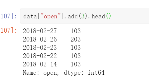
2.4.1算数运算
比如"open"这个一列数据全部加3
data["open"].add(3).head或者data["open"]+3
就是先索引到这一列然后再加三就行
如果里面的函数都统一的加减乘除的话可以data+3,data-3,data/3,data*3
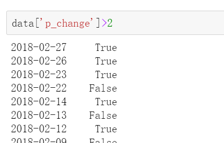
2.4.2逻辑运算
逻辑运算符号<、>、|、&
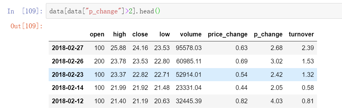
例如筛选p_change > 2的日期数据
data['p_change'] > 2返回带索引的布尔值
或者:data[data['p_chang']>2].head()
这个返回全部的
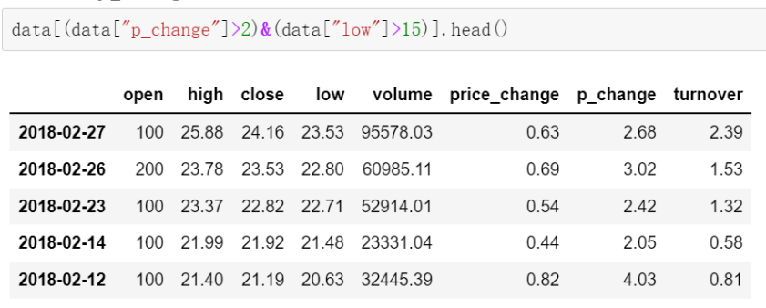
完成一个多个逻辑判断,筛选p_change > 2并且low > 15
data[(data["p_change"]>2)&(data["low"]>15)].head()
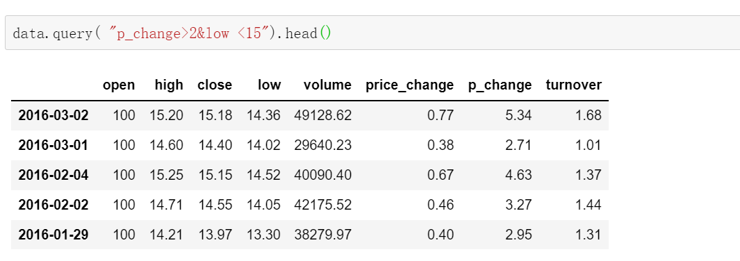
或者用逻辑运算函数
query(expr) expr是查询字符串
data.query( "p_change>2&low <15").head()
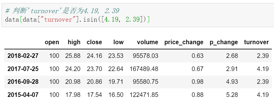
判断turnover'是否有4.19,2.39
data["turnover"].isin([4.19,2.39])
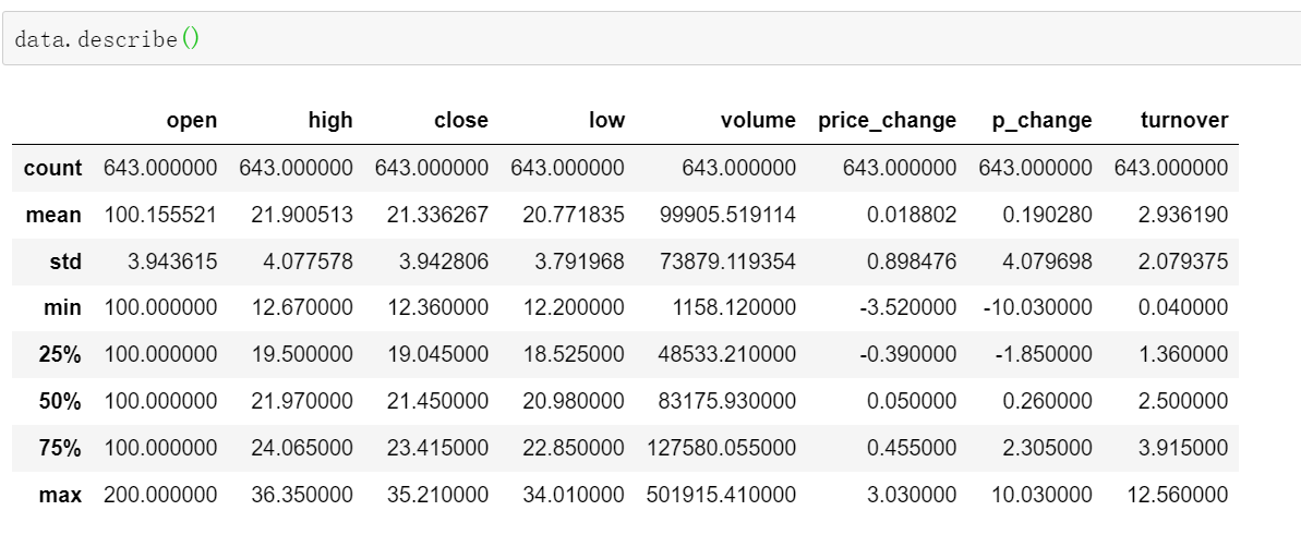
2.4.3统计运算
describe()
综合分析:能够直接得出很多统计结果,count , mean , std , min , max等
计算平均值、标准差、最大值、最小值
data.describe()
一些常用的API
例如:
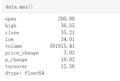
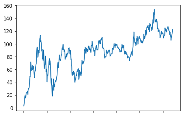
找所在位置是argmax和argmin
计算累加铜价函数cumsum()
data["p_change"].sort_index().cumsum().plot()
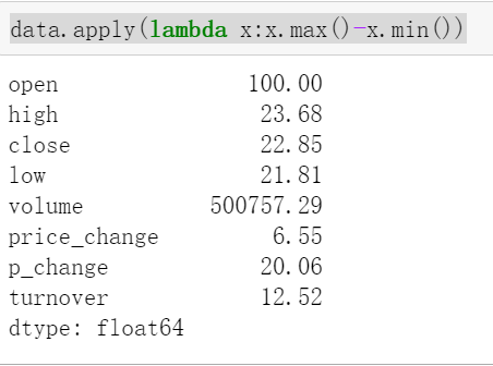
2.4.4自定义运算
apply(func,axis=O)
func:自定义函数
axis=O:默认是列,axis=1为行进行运算
例如:定义一个对列,最大值-最小值的函数
data.apply(lambda x:x.max()-x.min())
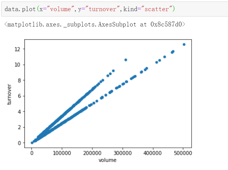
2.4pandas画图
pandas.DataFrame.plot
DataFrame.plot(x=None, y=None, kind='line',figsize=(,),fontsize=,colormap="")
----x: label or position, default None
----y: label, position or list of label, positions, default None
----Allows plotting of one column versus another
----kind: str
-------'line': line plot(default)
--------"bar": vertical bar plot
--------"barh": horizontal bar plot
--------"hist": histogram
--------"pie": pie plot
---------"scatter": scatter plot
----figsize是画布
----fontsize是字体大小
-----colormap是字体颜色
3.pandas的数据处理
请看这博客
4.pandas合并
4.1 pd.concat实现按方向合并
pd.concat([data1,data2],axis=1)按照行或列进行合并,axis=0为列索引,axis=1为行索引
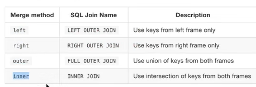
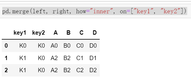
4.2 pd.merge()实现索引合并
pd.merge(left, right, how="inner", on=[索引]) on:索引
左连接,右连接,外连接,内连接
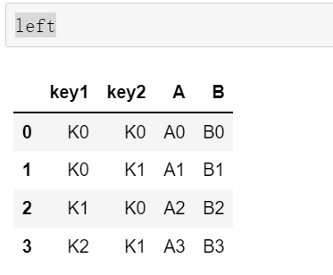
left = pd.DataFrame({'key1': ['K0', 'K0', 'K1', 'K2'],
'key2': ['K0', 'K1', 'K0', 'K1'],
'A': ['A0', 'A1', 'A2', 'A3'],
'B': ['B0', 'B1', 'B2', 'B3']})
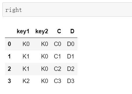
right = pd.DataFrame({'key1': ['K0', 'K1', 'K1', 'K2'],
'key2': ['K0', 'K0', 'K0', 'K0'],
'C': ['C0', 'C1', 'C2', 'C3'],
'D': ['D0', 'D1', 'D2', 'D3']})
pd.merge(left, right, how="inner", on=["key1", "key2"])
#内连接
5.分组和聚合

DataFrame.groupby(key,as_index=False)
key:分组的列数据,可以多个
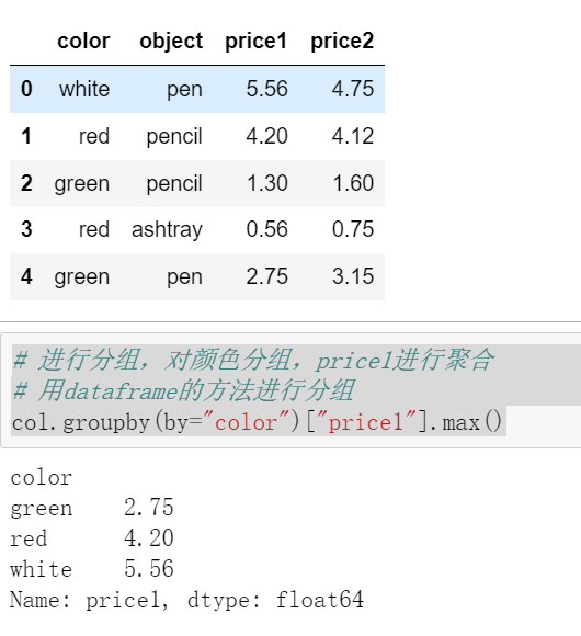
案例:不同颜色的不同笔的价格数据
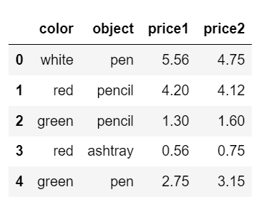
col =pd.DataFrame({'color': ['white','red','green','red','green'], 'object': ['pen','pencil','pencil','ashtray','pen'],
                   'price1':[5.56,4.20,1.30,0.56,2.75],'price2':[4.75,4.12,1.60,0.75,3.15]})
col
# 进行分组,对颜色分组,price1进行聚合,并求去每个分组的最大值
# 用dataframe的方法进行分组
col.groupby(by="color")["price1"].max()
6.交叉表与透视表
找到两个变量之间的关系
例如:
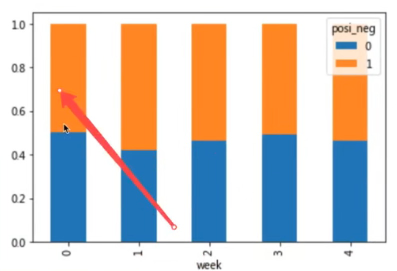
探究股票的涨跌与星期几有关?
以下图当中表示,week代表星期几,1,0代表这一天股票的涨跌幅是好还是坏,里面的数据代表比例
可以理解为所有时间为星期一等等的数据当中涨跌幅好坏的比例
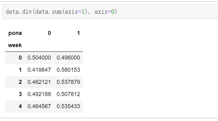
再这个图中:比如星期1,长得占0.419847,跌的占到0.580153
6.1交叉表
用于计算一列数据对于另外一列数据的分组个数(寻找两个列之间的关系)
pd.crosstab(value1, value2)
value1和value2是两个变量
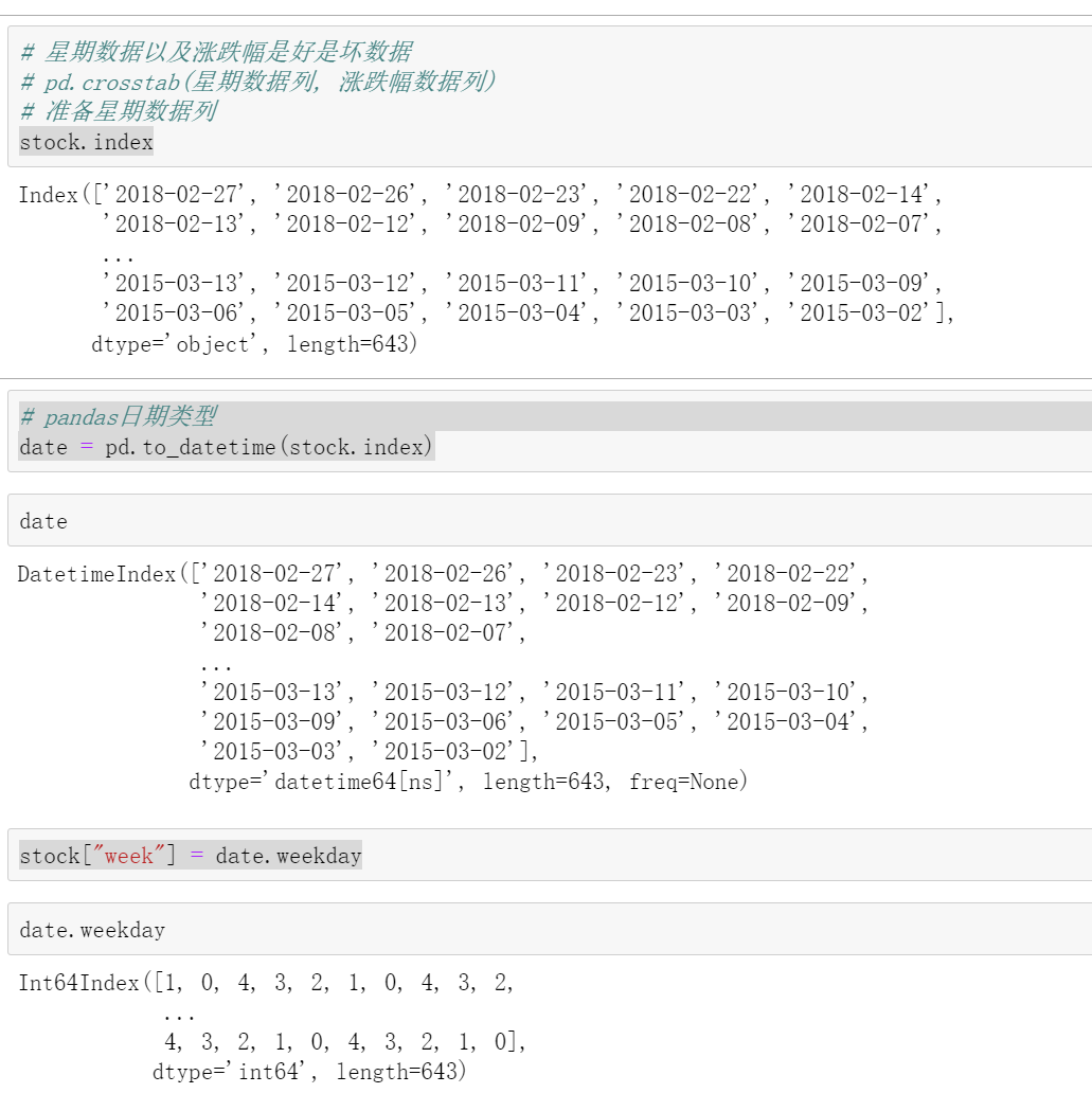
例如:星期数据以及涨跌幅是好是坏数据,就是上面的例子
pd.crosstab(星期数据列, 涨跌幅数据列)
准备星期数据列
准备星期数据列数据
stock.index
# 转化成pandas日期类型
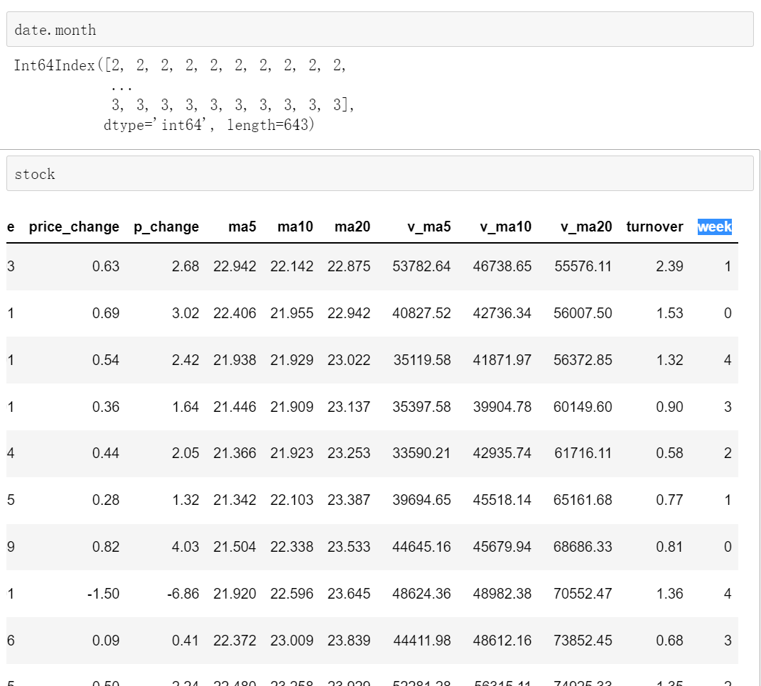
date = pd.to_datetime(stock.index)
#将stock中的哪一列替换掉
stock["week"] = date.weekday
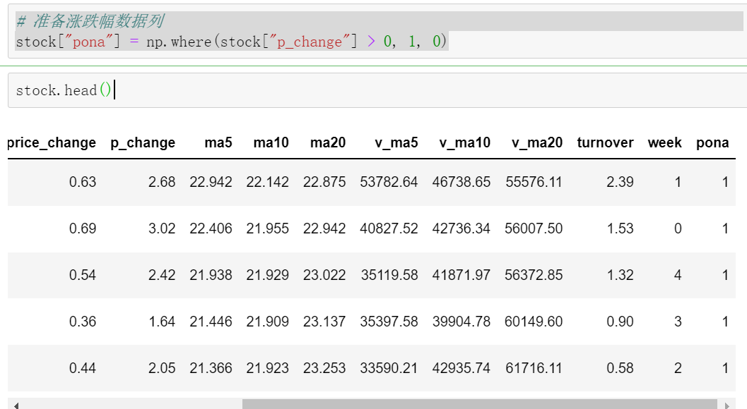
准备涨跌幅数据列
# 准备涨跌幅数据列,np.where(,,满足条件的,不满足条件的)
stock["pona"] = np.where(stock["p_change"] > 0, 1, 0)
交叉表
# 交叉表
data = pd.crosstab(stock["week"], stock["pona"])
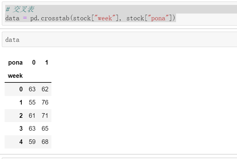
这个表里面就是星期一跌的有63个,涨的有62个
改造数据
因为原文中是百分比,所以我们要改变一下
data.div(data.sum(axis=1), axis=0)
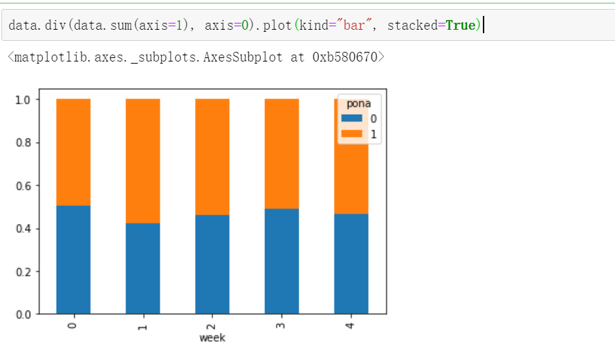
画图
data.div(data.sum(axis=1), axis=0).plot(kind="bar", stacked=True)
6.2透视表
DataFrame.pivot_table([], index=[])
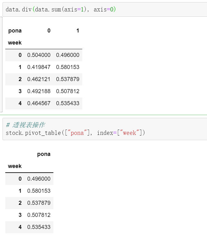
透视表更加简单就可以得出结果

 浙公网安备 33010602011771号