HybridSN 高光谱分类
HybridSN 高光谱分类
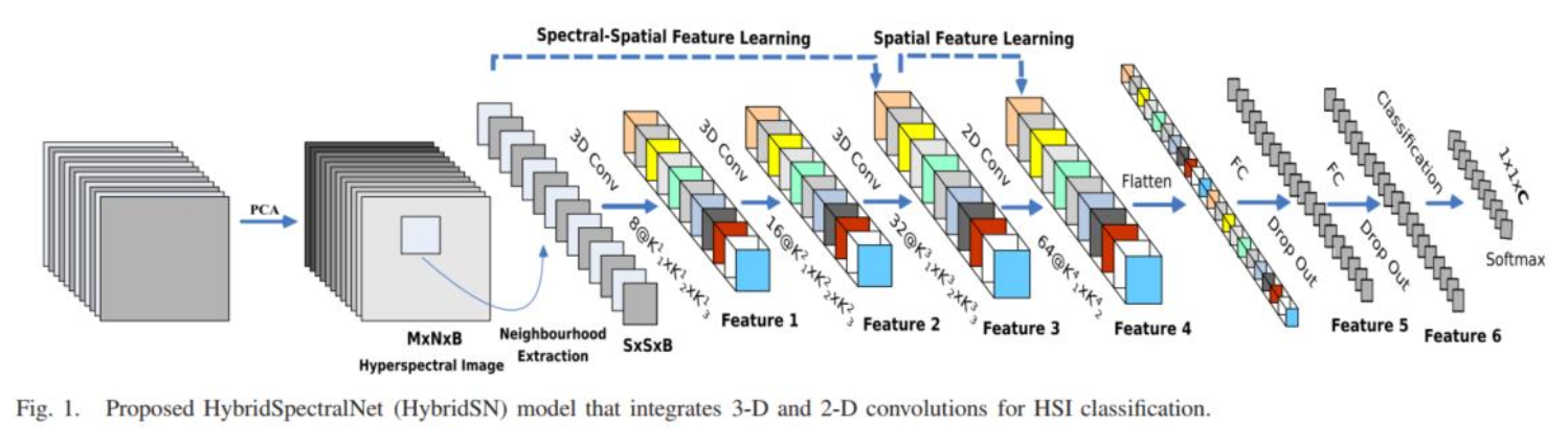
S. K. Roy, G. Krishna, S. R. Dubey, B. B. Chaudhuri HybridSN: Exploring 3-D–2-D CNN Feature Hierarchy for Hyperspectral Image Classification, IEEE GRSL 2020
这篇论文构建了一个 混合网络 解决高光谱图像分类问题,首先用 3D卷积,然后使用 2D卷积,代码相对简单,下面是代码的解析。
取得数据
! wget http://www.ehu.eus/ccwintco/uploads/6/67/Indian_pines_corrected.mat
! wget http://www.ehu.eus/ccwintco/uploads/c/c4/Indian_pines_gt.mat
! pip install spectral
引入基本函数
import numpy as np
import matplotlib.pyplot as plt
import scipy.io as sio
from sklearn.decomposition import PCA
from sklearn.model_selection import train_test_split
from sklearn.metrics import confusion_matrix, accuracy_score, classification_report, cohen_kappa_score
import spectral
import torch
import torchvision
import torch.nn as nn
import torch.nn.functional as F
import torch.optim as optim
定义 HybridSN 类
三维卷积部分:
- conv1:(1, 30, 25, 25), 8个 7x3x3 的卷积核 ==>(8, 24, 23, 23)
- conv2:(8, 24, 23, 23), 16个 5x3x3 的卷积核 ==>(16, 20, 21, 21)
- conv3:(16, 20, 21, 21),32个 3x3x3 的卷积核 ==>(32, 18, 19, 19)
接下来要进行二维卷积,因此把前面的 32*18 reshape 一下,得到 (576, 19, 19)
二维卷积:(576, 19, 19) 64个 3x3 的卷积核,得到 (64, 17, 17)
接下来是一个 flatten 操作,变为 18496 维的向量,
接下来依次为256,128节点的全连接层,都使用比例为0.4的 Dropout,
最后输出为 16 个节点,是最终的分类类别数。
下面是 HybridSN 类的代码
class_num = 16

class HybridSN(nn.Module):
  def __init__(self, num_classes=16):
    super(HybridSN, self).__init__()
    # conv1:(1, 30, 25, 25), 8个 7x3x3 的卷积核 ==>(8, 24, 23, 23)
    self.conv1 = nn.Conv3d(1, 8, (7, 3, 3))
    # conv2:(8, 24, 23, 23), 16个 5x3x3 的卷积核 ==>(16, 20, 21, 21)
    self.conv2 = nn.Conv3d(8, 16, (5, 3, 3))
    # conv3:(16, 20, 21, 21),32个 3x3x3 的卷积核 ==>(32, 18, 19, 19)
    self.conv3 = nn.Conv3d(16, 32, (3, 3, 3))
    # conv3_2d (576, 19, 19),64个 3x3 的卷积核 ==>((64, 17, 17)
    self.conv3_2d = nn.Conv2d(576, 64, (3,3))
    # 全连接层(256个节点)
    self.dense1 =  nn.Linear(18496,256)
    # 全连接层(128个节点)
    self.dense2 =  nn.Linear(256,128)
    # 最终输出层(16个节点)
    self.out = nn.Linear(128, num_classes)
    #  Dropout(0.4)
    self.drop = nn.Dropout(p=0.4)
    # 这是个坑, 下面细说
    # self.soft = nn.LogSoftmax(dim=1)
    # 激活函数ReLU
    self.relu = nn.ReLU()
  def forward(self, x):
    out = self.relu(self.conv1(x))
    out = self.relu(self.conv2(out))
    out = self.relu(self.conv3(out))
    # 进行二维卷积,因此把前面的 32*18 reshape 一下,得到 (576, 19, 19)
    out = out.view(-1, out.shape[1] * out.shape[2], out.shape[3], out.shape[4])
    out = self.relu(self.conv3_2d(out))
    # flatten 操作,变为 18496 维的向量,
    out = out.view(out.size(0), -1)
    out = self.dense1(out)
    out = self.drop(out)
    out = self.dense2(out)
    out = self.drop(out)
    out = self.out(out)
    out = self.soft(out)
    return out
当我第一次写完代码的时候,跑完发现准确率只有84%,并且avg loss一直不怎么下降。我仔细检查了 HybridSN类,通过增添bn层,发现效果也并不好。最终我把目标放在了唯一可能优化的地方,self.soft()。
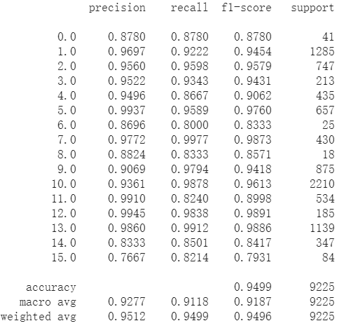
在第一次编写时,我是定义的softmax函数,即self.soft()=nn.softmax(),我在百度查询softmax时,发现了还有其他的例如logsoftmax,在使用logsoftmax代替softmax之后,效果显著提升,准确率稳定在96%以上。
那么为什么使用logsoftmax之后效果会好这么多呢???我也不知道,先挖个坑以后填。
经过反复测试和查阅资料找到原因了,其实不写self.soft()就能得到正确的准确率,多写了以后反而多此一举。
原因是 CrossEntropyLoss() = softmax + 负对数损失(已经包含了softmax) 。如果多写一次softmax,则结果会发生错误。
至于BN层的添加,我对conv3d,2d,混合都进行了添加,发现效果并不明显。。
# 随机输入,测试网络结构是否通
x = torch.randn(1, 1, 30, 25, 25)
net = HybridSN()
y = net(x)
print(y.shape)
'''
torch.Size([1, 16])
'''
创建数据集
首先对高光谱数据实施PCA降维;然后创建 keras 方便处理的数据格式;然后随机抽取 10% 数据做为训练集,剩余的做为测试集。
首先定义基本函数:
# 对高光谱数据 X 应用 PCA 变换
def applyPCA(X, numComponents):
    newX = np.reshape(X, (-1, X.shape[2]))
    pca = PCA(n_components=numComponents, whiten=True)
    newX = pca.fit_transform(newX)
    newX = np.reshape(newX, (X.shape[0], X.shape[1], numComponents))
    return newX

# 对单个像素周围提取 patch 时,边缘像素就无法取了,因此,给这部分像素进行 padding 操作
def padWithZeros(X, margin=2):
    newX = np.zeros((X.shape[0] + 2 * margin, X.shape[1] + 2* margin, X.shape[2]))
    x_offset = margin
    y_offset = margin
    newX[x_offset:X.shape[0] + x_offset, y_offset:X.shape[1] + y_offset, :] = X
    return newX

# 在每个像素周围提取 patch ,然后创建成符合 keras 处理的格式
def createImageCubes(X, y, windowSize=5, removeZeroLabels = True):
    # 给 X 做 padding
    margin = int((windowSize - 1) / 2)
    zeroPaddedX = padWithZeros(X, margin=margin)
    # split patches
    patchesData = np.zeros((X.shape[0] * X.shape[1], windowSize, windowSize, X.shape[2]))
    patchesLabels = np.zeros((X.shape[0] * X.shape[1]))
    patchIndex = 0
    for r in range(margin, zeroPaddedX.shape[0] - margin):
        for c in range(margin, zeroPaddedX.shape[1] - margin):
            patch = zeroPaddedX[r - margin:r + margin + 1, c - margin:c + margin + 1]
            patchesData[patchIndex, :, :, :] = patch
            patchesLabels[patchIndex] = y[r-margin, c-margin]
            patchIndex = patchIndex + 1
    if removeZeroLabels:
        patchesData = patchesData[patchesLabels>0,:,:,:]
        patchesLabels = patchesLabels[patchesLabels>0]
        patchesLabels -= 1
    return patchesData, patchesLabels

def splitTrainTestSet(X, y, testRatio, randomState=345):
    X_train, X_test, y_train, y_test = train_test_split(X, y, test_size=testRatio, random_state=randomState, stratify=y)
    return X_train, X_test, y_train, y_test
# 地物类别
class_num = 16
X = sio.loadmat('Indian_pines_corrected.mat')['indian_pines_corrected']
y = sio.loadmat('Indian_pines_gt.mat')['indian_pines_gt']

# 用于测试样本的比例
test_ratio = 0.90
# 每个像素周围提取 patch 的尺寸
patch_size = 25
# 使用 PCA 降维,得到主成分的数量
pca_components = 30

print('Hyperspectral data shape: ', X.shape)
print('Label shape: ', y.shape)

print('\n... ... PCA tranformation ... ...')
X_pca = applyPCA(X, numComponents=pca_components)
print('Data shape after PCA: ', X_pca.shape)

print('\n... ... create data cubes ... ...')
X_pca, y = createImageCubes(X_pca, y, windowSize=patch_size)
print('Data cube X shape: ', X_pca.shape)
print('Data cube y shape: ', y.shape)

print('\n... ... create train & test data ... ...')
Xtrain, Xtest, ytrain, ytest = splitTrainTestSet(X_pca, y, test_ratio)
print('Xtrain shape: ', Xtrain.shape)
print('Xtest  shape: ', Xtest.shape)

# 改变 Xtrain, Ytrain 的形状,以符合 keras 的要求
Xtrain = Xtrain.reshape(-1, patch_size, patch_size, pca_components, 1)
Xtest  = Xtest.reshape(-1, patch_size, patch_size, pca_components, 1)
print('before transpose: Xtrain shape: ', Xtrain.shape)
print('before transpose: Xtest  shape: ', Xtest.shape)

# 为了适应 pytorch 结构,数据要做 transpose
Xtrain = Xtrain.transpose(0, 4, 3, 1, 2)
Xtest  = Xtest.transpose(0, 4, 3, 1, 2)
print('after transpose: Xtrain shape: ', Xtrain.shape)
print('after transpose: Xtest  shape: ', Xtest.shape)


""" Training dataset"""
class TrainDS(torch.utils.data.Dataset):
    def __init__(self):
        self.len = Xtrain.shape[0]
        self.x_data = torch.FloatTensor(Xtrain)
        self.y_data = torch.LongTensor(ytrain)
    def __getitem__(self, index):
        # 根据索引返回数据和对应的标签
        return self.x_data[index], self.y_data[index]
    def __len__(self):
        # 返回文件数据的数目
        return self.len

""" Testing dataset"""
class TestDS(torch.utils.data.Dataset):
    def __init__(self):
        self.len = Xtest.shape[0]
        self.x_data = torch.FloatTensor(Xtest)
        self.y_data = torch.LongTensor(ytest)
    def __getitem__(self, index):
        # 根据索引返回数据和对应的标签
        return self.x_data[index], self.y_data[index]
    def __len__(self):
        # 返回文件数据的数目
        return self.len

# 创建 trainloader 和 testloader
trainset = TrainDS()
testset  = TestDS()
train_loader = torch.utils.data.DataLoader(dataset=trainset, batch_size=128, shuffle=True, num_workers=2)
test_loader  = torch.utils.data.DataLoader(dataset=testset,  batch_size=128, shuffle=False, num_workers=2)
模型训练
# 使用GPU训练,可以在菜单 "代码执行工具" -> "更改运行时类型" 里进行设置
device = torch.device("cuda:0" if torch.cuda.is_available() else "cpu")
# 网络放到GPU上
net = HybridSN().to(device)
criterion = nn.CrossEntropyLoss()
optimizer = optim.Adam(net.parameters(), lr=0.0005)
# 开始训练
total_loss = 0
for epoch in range(100):
for i, (inputs, labels) in enumerate(train_loader):
inputs = inputs.to(device)
labels = labels.to(device)
# 优化器梯度归零
optimizer.zero_grad()
# 正向传播 + 反向传播 + 优化
outputs = net(inputs)
loss = criterion(outputs, labels)
loss.backward()
optimizer.step()
total_loss += loss.item()
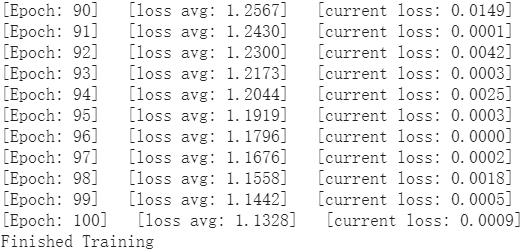
print('[Epoch: %d] [loss avg: %.4f] [current loss: %.4f]' %(epoch + 1, total_loss/(epoch+1), loss.item()))
print('Finished Training')
模型测试
count = 0
# 模型测试
for inputs, _ in test_loader:
    inputs = inputs.to(device)
    outputs = net(inputs)
    outputs = np.argmax(outputs.detach().cpu().numpy(), axis=1)
    if count == 0:
        y_pred_test =  outputs
        count = 1
    else:
        y_pred_test = np.concatenate( (y_pred_test, outputs) )

# 生成分类报告
classification = classification_report(ytest, y_pred_test, digits=4)
print(classification)

 浙公网安备 33010602011771号