RNN comprehension

RNN

https://www.tensorflow.org/tutorials/text/text_classification_rnn

Create the model

Above is a diagram of the model.

1. This model can be build as a tf.keras.Sequential.

2. The first layer is the encoder, which converts the text to a sequence of token indices.

3. After the encoder is an embedding layer. An embedding layer stores one vector per word. When called, it converts the sequences of word indices to sequences of vectors. These vectors are trainable. After training (on enough data), words with similar meanings often have similar vectors.

   This index-lookup is much more efficient than the equivalent operation of passing a one-hot encoded vector through a tf.keras.layers.Dense layer.

4. A recurrent neural network (RNN) processes sequence input by iterating through the elements. RNNs pass the outputs from one timestep to their input on the next timestep.

   The tf.keras.layers.Bidirectional wrapper can also be used with an RNN layer. This propagates the input forward and backwards through the RNN layer and then concatenates the final output.

   • The main advantage of a bidirectional RNN is that the signal from the beginning of the input doesn't need to be processed all the way through every timestep to affect the output.

   • The main disadvantage of a bidirectional RNN is that you can't efficiently stream predictions as words are being added to the end.

5. After the RNN has converted the sequence to a single vector the two layers.Dense do some final processing, and convert from this vector representation to a single logit as the classification output.

The code to implement this is below:

model = tf.keras.Sequential([
    encoder,
    tf.keras.layers.Embedding(
        input_dim=len(encoder.get_vocabulary()),
        output_dim=64,
        # Use masking to handle the variable sequence lengths
        mask_zero=True),
    tf.keras.layers.Bidirectional(tf.keras.layers.LSTM(64)),
    tf.keras.layers.Dense(64, activation='relu'),
    tf.keras.layers.Dense(1)
])

 

LSTM

https://towardsdatascience.com/illustrated-guide-to-lstms-and-gru-s-a-step-by-step-explanation-44e9eb85bf21

The Problem, Short-term Memory

Recurrent Neural Networks suffer from short-term memory. If a sequence is long enough, they’ll have a hard time carrying information from earlier time steps to later ones. So if you are trying to process a paragraph of text to do predictions, RNN’s may leave out important information from the beginning.

During back propagation, recurrent neural networks suffer from the vanishing gradient problem. Gradients are values used to update a neural networks weights. The vanishing gradient problem is when the gradient shrinks as it back propagates through time. If a gradient value becomes extremely small, it doesn’t contribute too much learning.

 

Gradient Update Rule

So in recurrent neural networks, layers that get a small gradient update stops learning. Those are usually the earlier layers. So because these layers don’t learn, RNN’s can forget what it seen in longer sequences, thus having a short-term memory. If you want to know more about the mechanics of recurrent neural networks in general, you can read my previous post here.

 

https://aditi-mittal.medium.com/understanding-rnn-and-lstm-f7cdf6dfc14e

What is Recurrent Neural Network (RNN)?

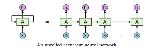
Recurrent Neural Network is a generalization of feedforward neural network that has an internal memory. RNN is recurrent in nature as it performs the same function for every input of data while the output of the current input depends on the past one computation. After producing the output, it is copied and sent back into the recurrent network. For making a decision, it considers the current input and the output that it has learned from the previous input.

Unlike feedforward neural networks, RNNs can use their internal state (memory) to process sequences of inputs. This makes them applicable to tasks such as unsegmented, connected handwriting recognition or speech recognition. In other neural networks, all the inputs are independent of each other. But in RNN, all the inputs are related to each other.

 

First, it takes the X(0) from the sequence of input and then it outputs h(0) which together with X(1) is the input for the next step. So, the h(0) and X(1) is the input for the next step. Similarly, h(1) from the next is the input with X(2) for the next step and so on. This way, it keeps remembering the context while training.

Word Embedding

https://towardsdatascience.com/introduction-to-word-embedding-and-word2vec-652d0c2060fa

Why do we need them?

Consider the following similar sentences: Have a good day and Have a great day. They hardly have different meaning. If we construct an exhaustive vocabulary (let’s call it V), it would have V = {Have, a, good, great, day}.

Now, let us create a one-hot encoded vector for each of these words in V. Length of our one-hot encoded vector would be equal to the size of V (=5). We would have a vector of zeros except for the element at the index representing the corresponding word in the vocabulary. That particular element would be one. The encodings below would explain this better.

Have = [1,0,0,0,0]`; a=[0,1,0,0,0]` ; good=[0,0,1,0,0]` ; great=[0,0,0,1,0]` ; day=[0,0,0,0,1]` (` represents transpose)

If we try to visualize these encodings, we can think of a 5 dimensional space, where each word occupies one of the dimensions and has nothing to do with the rest (no projection along the other dimensions). This means ‘good’ and ‘great’ are as different as ‘day’ and ‘have’, which is not true.

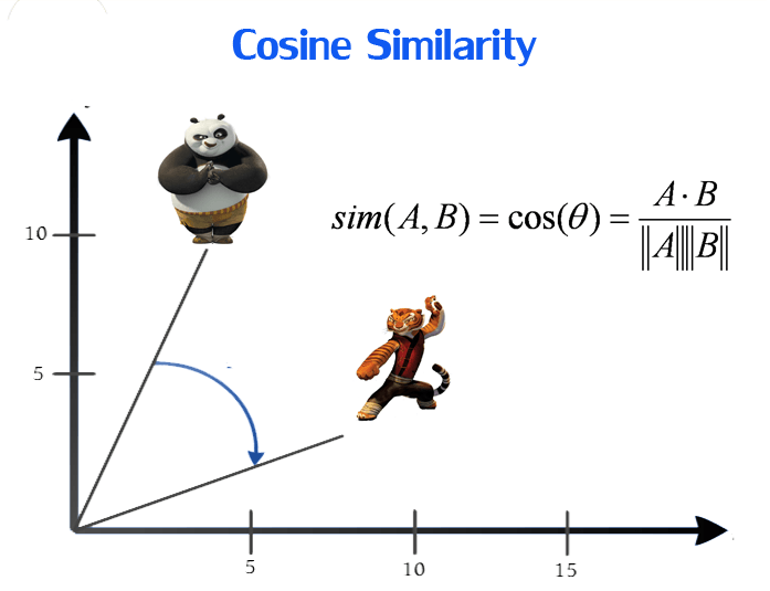
Our objective is to have words with similar context occupy close spatial positions. Mathematically, the cosine of the angle between such vectors should be close to 1, i.e. angle close to 0.

 

Google Images

Here comes the idea of generating distributed representations. Intuitively, we introduce some dependence of one word on the other words. The words in context of this word would get a greater share of this dependence. In one hot encoding representations, all the words are independent of each other, as mentioned earlier.

 

https://easyai.tech/ai-definition/word-embedding/

 

CBOW

https://thinkinfi.com/continuous-bag-of-words-cbow-single-word-model-how-it-works/

To implement Word2Vec, there are two flavors which are — Continuous Bag-Of-Words (CBOW) and continuous Skip-gram (SG). 

In this post I will explain only Continuous Bag of Word (CBOW) model with a one-word window to understand continuous bag of word (CBOW) clearly. If you can understand CBOW with single word model then multiword CBOW model will be so easy to you.

While explaining, I will present a few small examples with a text containing a few words. However, keep in mind that word2vec is typically trained with billions of words.

 

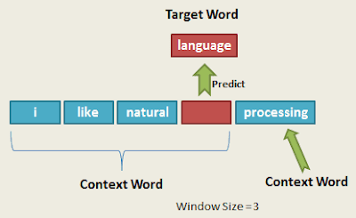
Continuous Bag of Words (CBOW):

It attempts to guess the output (target word) from its neighboring words (context words). You can think of it like fill in the blank task, where you need to guess word in place of blank by observing nearby words.