AGCN:Attention-driven Graph Clustering Network

论文阅读09-AGCN:Attention-driven Graph Clustering Network

论文信息

论文地址：https://dl.acm.org/doi/abs/10.1145/3474085.3475276

代码地址：ZhihaoPENG-CityU/MM21---AGCN：AGCN（注意力驱动的图聚类网络）的代码，被ACM MM 2021接受。 (github.com)

1.存在问题

1. 存在问题

传统卷积网络（即自编码器）与图卷积网络的结合在聚类中备受关注，其中自编码器提取节点属性特征，图卷积网络捕获拓扑图特征:

1. 缺乏灵活的组合机制来自适应融合这两种特征以学习判别表示.。：AE表示输入到GCN的 融合太过简单。
2. 忽略了嵌入在不同层的多尺度信息以用于后续的集群分配。：忽视每一层学习的表示信息，只利用最后一层的信息进行聚类

2. 解决问题

1. 如何解决

创新点：

1. AGCN 利用异质性融合模块动态融合节点属性特征和拓扑图特征
2. AGCN 开发了一个尺度融合模块来自适应地聚合嵌入在不同层的多尺度特征。

3.AGCN model

1. model structrue

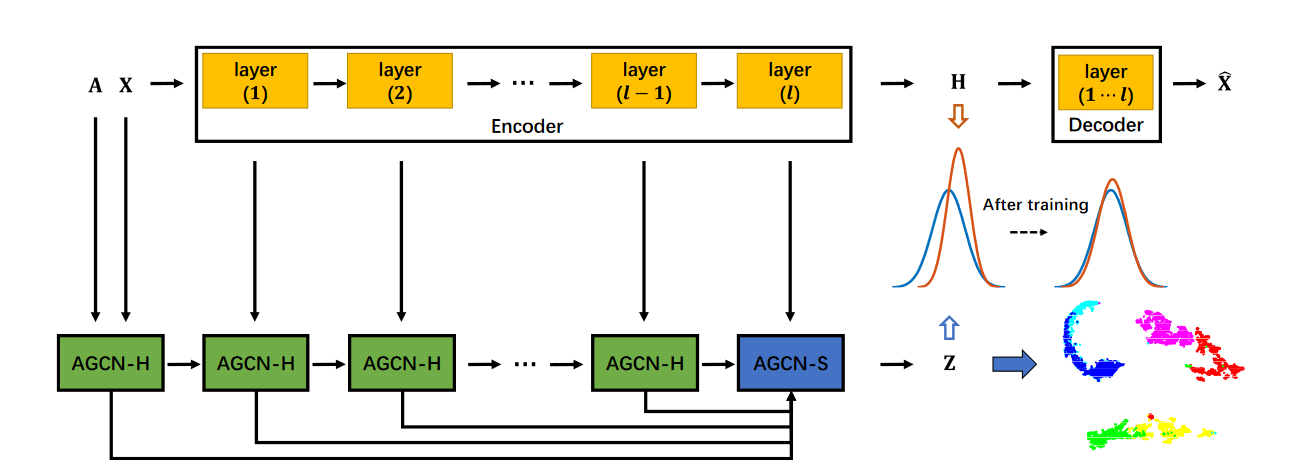
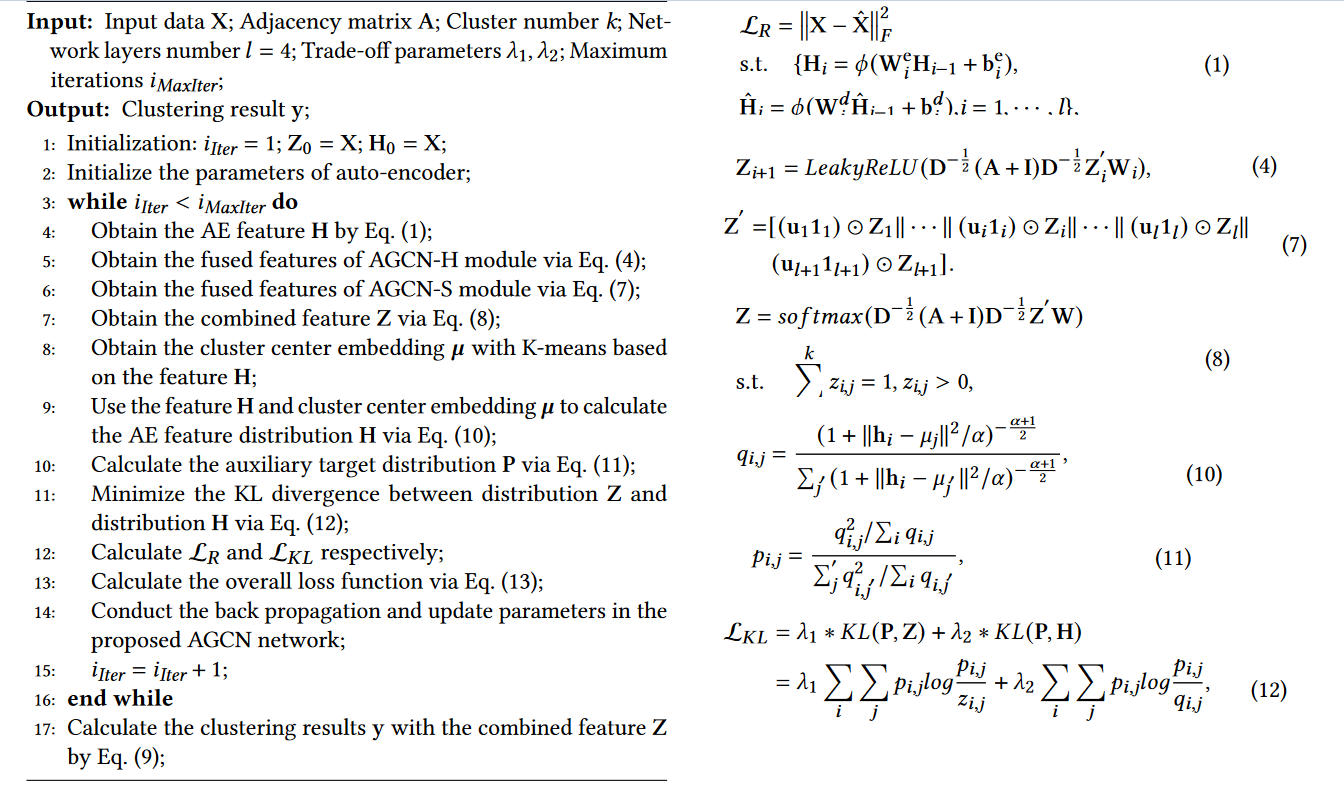
AGCN模型主要由3个模块组成：**AGCN-H模块， AGCN-S模块和联合监督****。

1. AGCN-H模块：AGCN-H 自适应合并来自同一层的 GCN 特征和 AE 特征。
2. AGCN-S模块： AGCN-S 动态连接来自不同层的多尺度特征
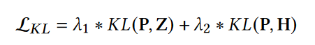
3. 联合监督模块：通过最小化 H 分布（如橙色所示）和 Z 分布（如蓝色所示）之间的 KL 散度来进行自我训练

2.AGCN-H：异质性融合模块

​ 由于图卷积网络（GCN）可以高效捕获拓扑图信息，自动编码器（AE）可以合理提取节点属性特征。 为了更好的融合二者，通过进行注意力系数学习和随后的加权特征融合，利用基于注意力的机制和异质性策略.

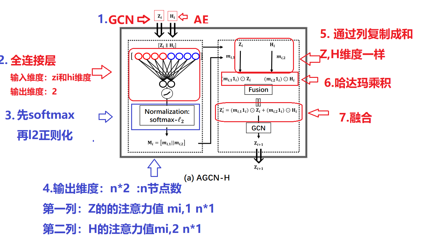
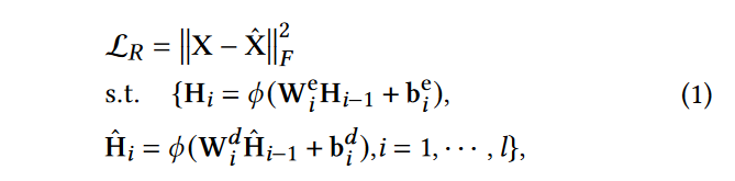
编码器-解码器模块用于通过最小化原始数据和重建数据之间的重建损失来提取潜在表示。

​

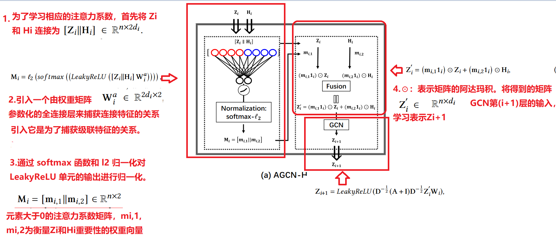
通过以上操作我们能够通过AGCN-H模块实现GCN和AE特征之间的动态特征融合.

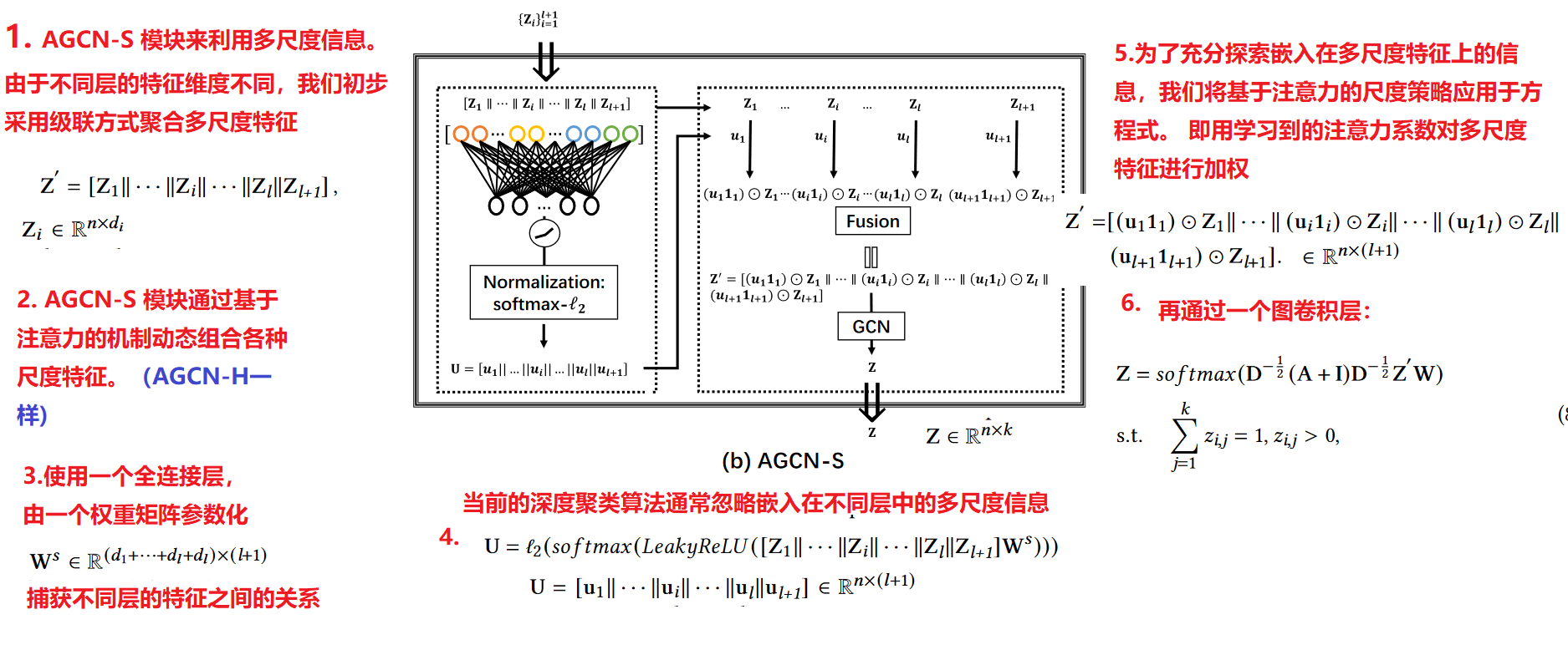
3.AGCN-S：尺度融合模块

​ 当前的深度聚类算法通常忽略嵌入在不同层中的多尺度信息.我们设计了 AGCN-S 模块来利用多尺度信息。由于不同层的特征维度不同，我们初步采用级联方式聚合多尺度特征

​

4. 联合监督模块

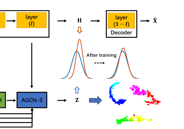
​ 我们使用学生 t 分布作为核来测量嵌入点和质心之间的相似性，其中测量的相似性可以解释为软分配:利用AE中的嵌入表示Z生成软分配P

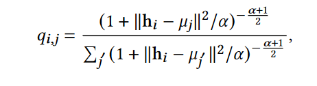
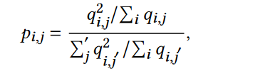
我们引入辅助目标分布 P 来避免崩溃问题:

​ 损失函数:

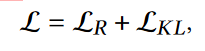
总损失函数:

5 . AGCN算法流程图

6.AGCN 代码

class AE(nn.Module):
    def __init__(self, n_enc_1, n_enc_2, n_enc_3, n_dec_1, n_dec_2, n_dec_3,
                 n_input, n_z):
        super(AE, self).__init__()
        # encoder
        self.enc_1 = Linear(n_input, n_enc_1)
        self.enc_2 = Linear(n_enc_1, n_enc_2)
        self.enc_3 = Linear(n_enc_2, n_enc_3)
        # extracted feature by AE
        self.z_layer = Linear(n_enc_3, n_z)
        # decoder
        self.dec_1 = Linear(n_z, n_dec_1)
        self.dec_2 = Linear(n_dec_1, n_dec_2)
        self.dec_3 = Linear(n_dec_2, n_dec_3)
        self.x_bar_layer = Linear(n_dec_3, n_input)
    def forward(self, x):
        enc_z2 = F.relu(self.enc_1(x))
        enc_z3 = F.relu(self.enc_2(enc_z2))
        enc_z4 = F.relu(self.enc_3(enc_z3))
        z = self.z_layer(enc_z4)
        dec_z2 = F.relu(self.dec_1(z))
        dec_z3 = F.relu(self.dec_2(dec_z2))
        dec_z4 = F.relu(self.dec_3(dec_z3))
        x_bar = self.x_bar_layer(dec_z4)

        return x_bar, enc_z2, enc_z3, enc_z4, z

class MLP_L(nn.Module):
    def __init__(self, n_mlp):
        super(MLP_L, self).__init__()
        self.wl = Linear(n_mlp, 5)# 5的原因:4层GCN 融和 和AE的嵌入表示
    def forward(self, mlp_in):
        weight_output = F.softmax(F.leaky_relu(self.wl(mlp_in)), dim=1)
        
        return weight_output

class MLP_1(nn.Module):
    def __init__(self, n_mlp):
        super(MLP_1, self).__init__()
        self.w1 = Linear(n_mlp,2)
    def forward(self, mlp_in):
        weight_output = F.softmax(F.leaky_relu(self.w1(mlp_in)), dim=1) 
        
        return weight_output

class MLP_2(nn.Module):
    def __init__(self, n_mlp):
        super(MLP_2, self).__init__()
        self.w2 = Linear(n_mlp, 2)
    def forward(self, mlp_in):
        weight_output = F.softmax(F.leaky_relu(self.w2(mlp_in)), dim=1)
        
        return weight_output

class MLP_3(nn.Module):
    def __init__(self, n_mlp):
        super(MLP_3, self).__init__()
        self.w3 = Linear(n_mlp, 2)
    def forward(self, mlp_in):
        weight_output = F.softmax(F.leaky_relu(self.w3(mlp_in)), dim=1)  
        
        return weight_output

class AGCN(nn.Module):

    def __init__(self, n_enc_1, n_enc_2, n_enc_3, n_dec_1, n_dec_2, n_dec_3, 
                n_input, n_z, n_clusters, v=1):
        super(AGCN, self).__init__()

        # AE
        self.ae = AE(
            n_enc_1=n_enc_1,
            n_enc_2=n_enc_2,
            n_enc_3=n_enc_3,
            n_dec_1=n_dec_1,
            n_dec_2=n_dec_2,
            n_dec_3=n_dec_3,
            n_input=n_input,
            n_z=n_z)
        self.ae.load_state_dict(torch.load(args.pretrain_path, map_location='cpu'))

        self.agcn_0 = GNNLayer(n_input, n_enc_1)
        self.agcn_1 = GNNLayer(n_enc_1, n_enc_2)
        self.agcn_2 = GNNLayer(n_enc_2, n_enc_3)
        self.agcn_3 = GNNLayer(n_enc_3, n_z)
        self.agcn_z = GNNLayer(3020,n_clusters)

        self.mlp = MLP_L(3020)

        # attention on [Z_i || H_i]
        self.mlp1 = MLP_1(2*n_enc_1)
        self.mlp2 = MLP_2(2*n_enc_2)
        self.mlp3 = MLP_3(2*n_enc_3)

        # cluster layer
        self.cluster_layer = Parameter(torch.Tensor(n_clusters, n_z))
        torch.nn.init.xavier_normal_(self.cluster_layer.data)

        # degree
        self.v = v

    def forward(self, x, adj):
        # AE Module
        x_bar, h1, h2, h3, z = self.ae(x)

        x_array = list(np.shape(x))
        n_x = x_array[0]

        # # AGCN-H
        z1 = self.agcn_0(x, adj)
        # z2
        m1 = self.mlp1( torch.cat((h1,z1), 1) )# 1,表示按照列拼接
        m1 = F.normalize(m1,p=2)# 
        m11 = torch.reshape(m1[:,0], [n_x, 1])# 将torch.reshape(x,y)将x形状转为y
        m12 = torch.reshape(m1[:,1], [n_x, 1])
        m11_broadcast =  m11.repeat(1,500)# 行*1 列乘以500 进行复制
        m12_broadcast =  m12.repeat(1,500)
        z2 = self.agcn_1( m11_broadcast.mul(z1)+m12_broadcast.mul(h1), adj)#融合传入gcn传播
        # z3
        m2 = self.mlp2( torch.cat((h2,z2),1) )     
        m2 = F.normalize(m2,p=2)
        m21 = torch.reshape(m2[:,0], [n_x, 1])
        m22 = torch.reshape(m2[:,1], [n_x, 1])
        m21_broadcast = m21.repeat(1,500)
        m22_broadcast = m22.repeat(1,500)
        z3 = self.agcn_2( m21_broadcast.mul(z2)+m22_broadcast.mul(h2), adj)
        # z4
        m3 = self.mlp3( torch.cat((h3,z3),1) )# self.mlp3(h2)      
        m3 = F.normalize(m3,p=2)
        m31 = torch.reshape(m3[:,0], [n_x, 1])
        m32 = torch.reshape(m3[:,1], [n_x, 1])
        m31_broadcast = m31.repeat(1,2000)
        m32_broadcast = m32.repeat(1,2000)
        z4 = self.agcn_3( m31_broadcast.mul(z3)+m32_broadcast.mul(h3), adj)

        # # AGCN-S
        u  = self.mlp(torch.cat((z1,z2,z3,z4,z),1))# 和前面一样
        u = F.normalize(u,p=2) 
        u0 = torch.reshape(u[:,0], [n_x, 1])
        u1 = torch.reshape(u[:,1], [n_x, 1])
        u2 = torch.reshape(u[:,2], [n_x, 1])
        u3 = torch.reshape(u[:,3], [n_x, 1])
        u4 = torch.reshape(u[:,4], [n_x, 1])

        tile_u0 = u0.repeat(1,500)
        tile_u1 = u1.repeat(1,500)
        tile_u2 = u2.repeat(1,2000)
        tile_u3 = u3.repeat(1,10)
        tile_u4 = u4.repeat(1,10)

        net_output = torch.cat((tile_u0.mul(z1), tile_u1.mul(z2), tile_u2.mul(z3), tile_u3.mul(z4), tile_u4.mul(z)), 1 )   
        net_output = self.agcn_z(net_output, adj, active=False) 
        predict = F.softmax(net_output, dim=1)# 和sdcn 一样 n*cluster
        q = 1.0 / (1.0 + torch.sum(torch.pow(z.unsqueeze(1) - self.cluster_layer, 2), 2) / self.v)#利用AE嵌入表示生成软分配 q
        q = q.pow((self.v + 1.0) / 2.0)
        q = (q.t() / torch.sum(q, 1)).t()

        """
        xbar: AE重构特征矩阵
        q:AE的嵌入表示 生成软分配q
        predict:sdcn 中直接生成聚类目标 n*cluster
        z:AE 嵌入表示 n*10
        net_output:融合多个层级 n*3020
        """
        
        return x_bar, q, predict, z, net_output

4. result Analysis

1. 数据集

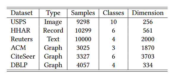
2. 实验结果

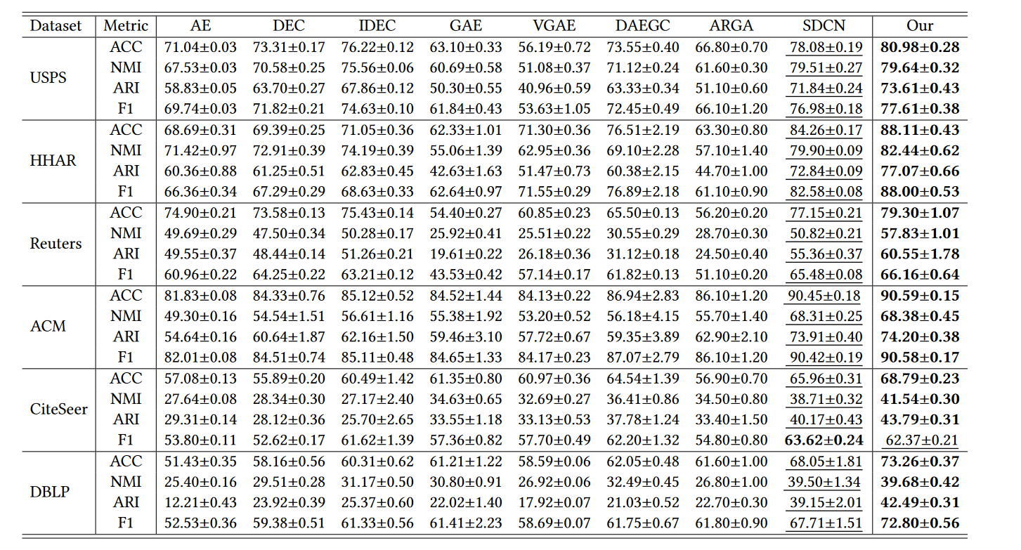
3.实验结果分析

1. 我们的方法自适应地融合了 GCN 特征和 AE 特征，以利用大量有鉴别力的信息作为尽可能。
2. 我们的方法动态结合多尺度特征以充分利用每一层的信息。
3. 我们设计的训练策略可以通过提供丰富且有辨别力的信息来构建软分配，从而为聚类开发更强大的指导。
4. DAEGC 比 GAE 表现更好，验证了考虑基于注意力的机制的重要性。通过将基于注意力的机制扩展到异质性和尺度特征融合，我们的 AGCN-H 和 AGCNS 模块能够进一步显着提高性能
5. SDCN 的性能优于基于 AE 的聚类方法（AE、DEC、IDEC）和基于 GCN 的方法（GAE、VGAE、ARGA），验证了将 AE 和 GCN 模型结合在一起的重要性。然而，SDCN将图结构特征和节点属性特征的重要性等同起来，忽略了多尺度特征，导致聚类性能欠佳

4. 消融实验:ablation

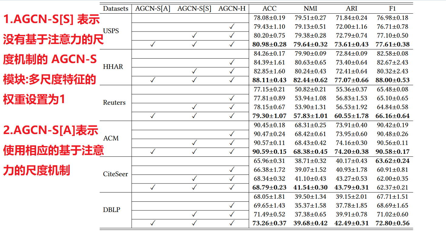
AGCN-H模块分析:

首先检查 AGCN-H 模块，其中实验比较显示在表 4 中每个数据集的第一行（没有 AGCN-H 模块）和第二行（有 AGCN-H 模块）。我们可以观察到AGCN-H模块在一定程度上产生了性能提升，验证了基于attention的heterogeneity-wise策略的有效性，即利用动态加权机制学习灵活的表示有利于获得更好的聚类结果

AGCN-S模块分析:

我们从两个方面评估 AGCN-S 模块:包括（i）多尺度特征融合（标记为 AGCN-S[S]）和（ii）基于注意力的尺度策略（标记为 AGCN-S[ A]）

对于第一个方面，通过比较表4中每个数据集第二行和第三行所示的实验结果，我们可以发现多尺度特征融合在大多数情况下有助于获得更好的聚类性能.

对于第二个方面，通过比较表4中第三行和第四行的每个数据集结果，我们可以发现考虑基于注意力的scale-wise策略能够获得最好的聚类性能。