OpenCV笔记（4）(直方图、傅里叶变换、高低通滤波)

一、直方图

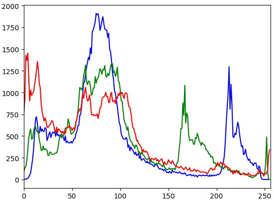
用于统计图片中各像素值：

# 画一个图像各通道的直方图
def draw_hist(img):
    color = ('b', 'g', 'r')
    for i, col in enumerate(color):
        hist = cv.calcHist([img], [i], None, [256], [0, 256])
        # print(hist.shape)
        plt.plot(hist, color=col)
        plt.xlim([0, 256])
    plt.show()

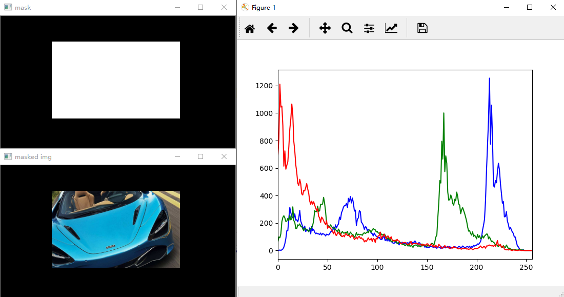
计算直方图时使用mask：

# 使用掩码
def draw_hist_with_mask(img):
    mask = np.zeros(img.shape[:2], np.uint8)
    mask[50:200, 100:350] = 255
    cv.imshow('mask', mask)
    
    # 将掩码转换为bool类型
    bi_mask = (mask == 255)
    # 将掩码作用于原图上
    cv.imshow('masked img', img * bi_mask[:, :, np.newaxis])

    color = ('b', 'g', 'r')
    for i, col in enumerate(color):
        # 使用mask，只计算mask中的像素的直方图
        hist = cv.calcHist([img], [i], mask, [256], [0, 256])
        # print(hist.shape)
        plt.plot(hist, color=col)
        plt.xlim([0, 256])
    plt.show()

 直方图均衡：

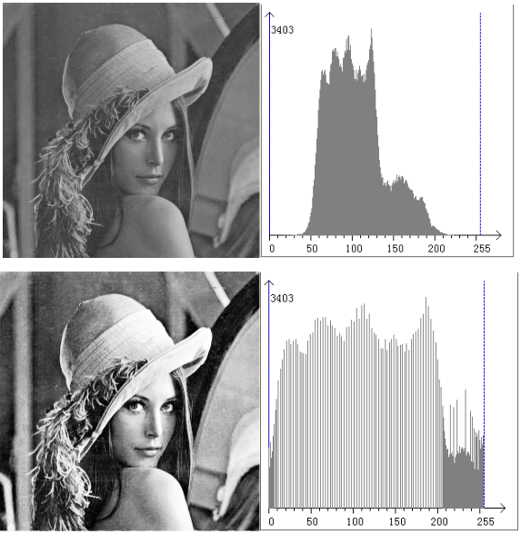
# 直方图均衡
def equal_hist(image):
    image = cv.cvtColor(image, cv.COLOR_RGB2GRAY)
    equ = cv.equalizeHist(image)
    plt.hist(image.ravel(), 256)
    plt.hist(equ.ravel(), 256)
    plt.show()

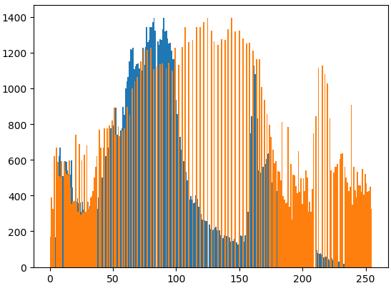
图中蓝色部分为原图的直方图，橙色部分为均衡后的直方图，均衡前后的效果如下图所示：

CLAHE（限制对比度自适应直方图均衡）：

# 自适应直方图均衡化
def CLAHE_proc(image):
    'CLAHE:限制对比度自适应直方图均衡'
    # 先转换为灰度图像
    image = cv.cvtColor(image, cv.COLOR_RGB2GRAY)
    # 创建CLAHE分块
    clahe = cv.createCLAHE(clipLimit=2.0, tileGridSize=(8, 8))
    # 执行CLAHE均衡化
    res_clahe = clahe.apply(image)
    cv.imshow('res_clahe', res_clahe)
    
    # 对比普通均衡化
    equ = cv.equalizeHist(image)
    cv.imshow('equ', equ)

左图为CLAHE效果，右图为普通均衡化效果。CLAHE可以减少过爆或过暗，因为他不是基于整张图片来均衡。

二、傅里叶变换

通过傅里叶变换，我们可以将图像从空间域转换到频率域，然后在频率域中对其进行滤波，主要有高通滤波和低通滤波。

概念：

　　高频：变化剧烈的灰度分量，例如边界

　　低频：变化缓慢的灰度分量

　　高通滤波器：只保留高频，过滤出边界

　　低通滤波器：只保留低频，使图像变模糊

 

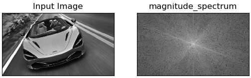
空间域转频率域：

# 将图像从空间域转换为频率域
def fourier_trans(img):
    # 使用灰度图像
    img = cv.cvtColor(img, cv.COLOR_RGB2GRAY)
    # uint8转换为float32
    img_float32 = np.float32(img)
    # 傅里叶转换为复数
    dft = cv.dft(img_float32, flags=cv.DFT_COMPLEX_OUTPUT)
    # 将低频从左上角转换到中心
    dft_shift = np.fft.fftshift(dft)
    # 转换为可以显示的图片（频谱图）
    magnitude_spectrum = 20 * np.log(cv.magnitude(dft_shift[:, :, 0], dft_shift[:, :, 1]))

    # 使用plt展示原图的灰度图
    plt.subplot(121)
    plt.imshow(img, cmap='gray')
    plt.title('Input Image')
    plt.xticks([])
    plt.yticks([])
    # 展示频谱图
    plt.subplot(122)
    plt.imshow(magnitude_spectrum, cmap='gray')
    plt.title('magnitude_spectrum')
    plt.xticks([])
    plt.yticks([])
    plt.show()

频率域转回空间域（并实验低通和高通滤波）：

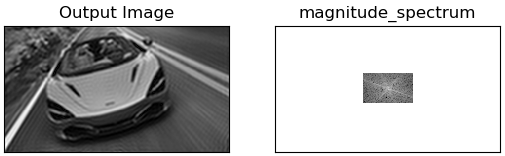
低频滤波：

# 从频率域转换回空间域（并使用低通滤波）
def fourier_trans_back(img):
    # 使用灰度图像
    img = cv.cvtColor(img, cv.COLOR_RGB2GRAY)
    # uint8转换为float32
    img_float32 = np.float32(img)
    # 傅里叶转换为复数
    dft = cv.dft(img_float32, flags=cv.DFT_COMPLEX_OUTPUT)
    # 将低频从左上角转换到中心
    dft_shift = np.fft.fftshift(dft)

    # 在这里进行低通滤波
    rows, cols = img.shape
    c_row, c_col = int(rows / 2), int(cols / 2)
    mask_low = np.zeros_like(dft_shift, np.uint8)
    mask_low[c_row - 30:c_row + 30, c_col - 50:c_col + 50] = 1
    # 使用低通滤波
    fshift_low = dft_shift * mask_low
    # 转换为可以显示的图片（fshift_low），fshift_low中包含实部和虚部
    magnitude_spectrum_low = 20 * np.log(cv.magnitude(fshift_low[:, :, 0], fshift_low[:, :, 1]))

    f_ishift_low = np.fft.ifftshift(fshift_low)
    img_back_low = cv.idft(f_ishift_low)
    img_back_low = cv.magnitude(img_back_low[:, :, 0], img_back_low[:, :, 1])

    # 使用plt低通滤波后的图像
    plt.subplot(121)
    plt.imshow(img_back_low, cmap='gray')
    plt.title('Output Image')
    plt.xticks([])
    plt.yticks([])
    # 展示低通滤波后的频谱图
    plt.subplot(122)
    plt.imshow(magnitude_spectrum_low, cmap='gray')
    plt.title('magnitude_spectrum')
    plt.xticks([])
    plt.yticks([])
    plt.show()

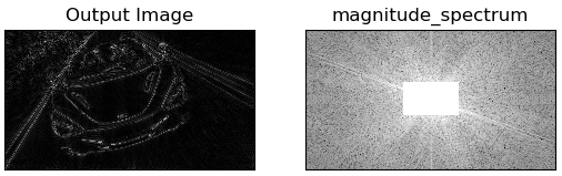
高频滤波：

# 从频率域转换回空间域（并使用高通滤波）
def fourier_trans_back(img):
    # 使用灰度图像
    img = cv.cvtColor(img, cv.COLOR_RGB2GRAY)
    # uint8转换为float32
    img_float32 = np.float32(img)
    # 傅里叶转换为复数
    dft = cv.dft(img_float32, flags=cv.DFT_COMPLEX_OUTPUT)
    # 将低频从左上角转换到中心
    dft_shift = np.fft.fftshift(dft)

    # 在这里进行高通滤波
    rows, cols = img.shape
    c_row, c_col = int(rows / 2), int(cols / 2)
    mask_high = np.ones_like(dft_shift, np.uint8)
    mask_high[c_row - 30:c_row + 30, c_col - 50:c_col + 50] = 0
    # 使用高通滤波
    fshift_high = dft_shift * mask_high
    # 转换为可以显示的图片（fshift_high），fshift_high中包含实部和虚部
    magnitude_spectrum_high = 20 * np.log(cv.magnitude(fshift_high[:, :, 0], fshift_high[:, :, 1]))

    f_ishift_high = np.fft.ifftshift(fshift_high)
    img_back_high = cv.idft(f_ishift_high)
    img_back_high = cv.magnitude(img_back_high[:, :, 0], img_back_high[:, :, 1])

    # 使用plt高通滤波后的图像
    plt.subplot(121)
    plt.imshow(img_back_high, cmap='gray')
    plt.title('Output Image')
    plt.xticks([])
    plt.yticks([])
    # 展示高通滤波后的频谱图
    plt.subplot(122)
    plt.imshow(magnitude_spectrum_high, cmap='gray')
    plt.title('magnitude_spectrum')
    plt.xticks([])
    plt.yticks([])
    plt.show()